
In the field of statistics and probability theory, the covariance matrix is a fundamental concept used to understand the relationships and variability between variables in a dataset. It is also known as the variance-covariance matrix, as it contains information about both the variances of individual variables and the covariances between pairs of variables.
The covariance matrix is a square matrix, where the diagonal elements represent the variances of the variables, and the off-diagonal elements represent the covariances between pairs of variables. It provides a comprehensive summary of how the variables in a dataset vary together, as well as the strength and direction of their relationships.
Understanding the covariance matrix is essential in various statistical techniques and applications. It is commonly used in multivariate analysis, portfolio optimization, risk management, and machine learning algorithms such as principal component analysis (PCA) and linear regression.
In the following sections, we will delve deeper into the concept of covariance matrix, including its definition, properties, calculation methods, and practical examples.
What is the Covariance Matrix?
The covariance matrix, denoted by Σ or C, is a square matrix that captures the covariance values between variables in a dataset. It provides a comprehensive view of the relationships and variability between variables, allowing us to better understand the structure of the dataset.
The covariance between two variables measures how they vary together. A positive covariance indicates a positive relationship, meaning that when one variable increases, the other variable tends to increase as well. A negative covariance indicates a negative relationship, where an increase in one variable corresponds to a decrease in the other variable. A covariance of zero suggests no linear relationship between the variables.
The covariance matrix extends this concept to multiple variables in a dataset. It represents the variances of individual variables along the diagonal elements and the covariances between pairs of variables in the off-diagonal elements. By examining the values in the covariance matrix, we can gain insights into the interdependencies and patterns within the dataset.
Variance and Covariance Matrix
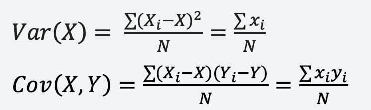
The variance of a single variable measures the spread or variability of that variable. It is the average of the squared deviations from the mean. The variance of a variable X is denoted as Var(X) and can be calculated using the following formula:
Var(X) = Σ (Xi – X)^2 / N
Where Xi represents the individual data points, X represents the mean of the dataset, and N is the total number of data points.
Covariance, on the other hand, measures how two variables vary together. It is the average of the products of the deviations of each variable from their respective means. The covariance between two variables X and Y is denoted as Cov(X, Y) and can be calculated using the following formula:
Cov(X, Y) = Σ (Xi – X)(Yi – Y) / N
Where Xi and Yi represent the individual data points for variables X and Y, and X and Y represent the means of the respective variables.
The variance and covariance values are then organized into a matrix form, creating the covariance matrix. This matrix provides a comprehensive summary of the variability and relationships between variables in the dataset.
How to Calculate Covariance Matrix?
To calculate the covariance matrix, we need to follow a step-by-step process. Let’s assume we have a dataset with n variables and m observations.
- Calculate the mean for each variable by summing up the values for that variable and dividing by the number of observations.
- Create a deviation matrix by subtracting the mean of each variable from the corresponding values.
- Calculate the covariance between each pair of variables by multiplying the deviations of the two variables and summing them up for each observation. Divide this sum by the number of observations.
- Organize the variance and covariance values into a matrix form, with the variances along the diagonal and the covariances in the off-diagonal elements.
The resulting matrix is the covariance matrix, which provides a comprehensive view of the relationships and variability between variables in the dataset.
.png)
Covariance Matrix Formula
The general formula for the covariance matrix, denoted as Σ or C, can be expressed as follows:
Σ = [ Cov(X1, X1) Cov(X1, X2) … Cov(X1, Xn) Cov(X2, X1) Cov(X2, X2) … Cov(X2, Xn) … Cov(Xn, X1) Cov(Xn, X2) … Cov(Xn, Xn) ]
Where Cov(Xi, Xj) represents the covariance between variables Xi and Xj.
The covariance matrix is a square matrix of size n x n, where n is the number of variables in the dataset. The diagonal elements of the matrix represent the variances of the individual variables, while the off-diagonal elements represent the covariances between pairs of variables.
Algorithm for Covariance Matrix
To calculate the covariance matrix, we can follow the algorithm outlined below:
- Calculate the mean vector μ of the dataset by finding the mean for each variable.
- Create a deviation matrix X by subtracting the mean vector μ from each observation in the dataset.
- Calculate the covariance matrix Σ by multiplying the transpose of the deviation matrix X with itself and dividing by the number of observations.
Σ = (1 / n) * X^T * X
Where X^T represents the transpose of the deviation matrix X and n is the number of observations in the dataset.
The resulting matrix Σ is the covariance matrix, which provides information about the variability and relationships between variables in the dataset.
Properties of Covariance Matrix
The covariance matrix has several important properties that make it a valuable tool in statistical analysis. These properties include:
- Symmetry: The covariance matrix is always symmetric, meaning that the element in the ith row and jth column is equal to the element in the jth row and ith column.
- Positive Semi-definiteness: The covariance matrix is positive semi-definite, which means that all its eigenvalues are non-negative.
- Diagonal Elements: The diagonal elements of the covariance matrix represent the variances of the individual variables. They are always non-negative.
- Off-diagonal Elements: The off-diagonal elements of the covariance matrix represent the covariances between pairs of variables. They can be positive, negative, or zero, depending on the relationship between the variables.
- Eigenvalues and Eigenvectors: The eigenvalues and eigenvectors of the covariance matrix provide insights into the variability and relationships between variables. The eigenvectors represent the directions of maximum variability, while the eigenvalues represent the amount of variability in each direction.
- Determinant: The determinant of the covariance matrix provides information about the overall variability of the dataset. If the determinant is zero, it indicates that the variables are linearly dependent.
- Inverse: The inverse of the covariance matrix, if it exists, is called the precision matrix or concentration matrix. It is useful in various statistical calculations and inference.
Understanding these properties is crucial in interpreting and analyzing the covariance matrix in statistical analysis and modeling.
Covariance Matrix Structure
The structure of the covariance matrix is defined by the variances and covariances between variables in a dataset. It is a square matrix, where the diagonal elements represent the variances of the individual variables, and the off-diagonal elements represent the covariances between pairs of variables.
The covariance matrix can be written in the following form:
Σ = [ Var(X1) Cov(X1, X2) … Cov(X1, Xn) Cov(X2, X1) Var(X2) … Cov(X2, Xn) … Cov(Xn, X1) Cov(Xn, X2) … Var(Xn) ]
Where Var(Xi) represents the variance of variable Xi, and Cov(Xi, Xj) represents the covariance between variables Xi and Xj.
The diagonal elements of the covariance matrix represent the variances of the individual variables, while the off-diagonal elements represent the covariances between pairs of variables. The structure of the covariance matrix provides important information about the relationships and variability between variables in a dataset.
Linear Transformations of the Data Set
Linear transformations can also be applied to the data set, and the covariance matrix can help understand these transformations. Suppose we have a random vector X and we apply a linear transformation A to it to get a new vector Y = AX. The covariance matrix of Y can be obtained from the covariance matrix of X by the transformation:
[Cov(Y) = A * Cov(X) * A^T]
where A is the transformation matrix and A^T its transpose. This property is useful in many applications, including principal component analysis, where the data is transformed to a new coordinate system.
Eigen Decomposition of the Covariance Matrix
The eigen decomposition of the covariance matrix is a powerful tool in multivariate analysis. It provides insights into the variability and relationships between variables in a dataset by expressing the covariance matrix as a product of eigenvectors and eigenvalues.
The eigen decomposition of the covariance matrix Σ can be written as follows:
Σ = VΛV^T
Where V is a matrix whose columns are the eigenvectors of Σ, and Λ is a diagonal matrix whose diagonal elements are the eigenvalues of Σ.
The eigenvectors represent the directions of maximum variability in the dataset, while the eigenvalues represent the amount of variability in each direction. The eigenvectors are orthogonal to each other, meaning that they are perpendicular and do not share any common direction of variability.
The eigen decomposition allows us to transform the dataset into a new coordinate system defined by the eigenvectors. This transformation is known as principal component analysis (PCA) and is used to reduce the dimensionality of the dataset while preserving the most important information.
By analyzing the eigenvalues, we can determine the proportion of variability explained by each eigenvector and select the most influential eigenvectors for further analysis.
Correlation Matrix vs. Covariance Matrix
The correlation matrix and covariance matrix are closely related but capture different aspects of the relationships between variables in a dataset.
The correlation matrix represents the correlations between variables, which are standardized measures of the linear relationships. Correlation values range from -1 to 1, with -1 indicating a perfect negative linear relationship, 1 indicating a perfect positive linear relationship, and 0 indicating no linear relationship.
On the other hand, the covariance matrix represents the covariances between variables, which are measures of the linear relationships without standardization. Covariance values can be positive, negative, or zero, indicating the strength and direction of the linear relationship.
The correlation matrix is obtained by dividing the covariance matrix by the product of the standard deviations of the variables. This standardization allows for easier interpretation and comparison of the relationships between variables.
While the covariance matrix provides information about the variability and relationships between variables in their original units, the correlation matrix allows for a standardized comparison of the strength and direction of the relationships.
Both the correlation matrix and covariance matrix are useful in statistical analysis, depending on the specific goals and context of the analysis.
Frequently Asked Questions About Covariance Matrix
How to Read a Covariance Matrix?
Reading a covariance matrix involves understanding the structure of the matrix and interpreting the values in the diagonal and off-diagonal elements.
The diagonal elements represent the variances of the individual variables. A larger value indicates higher variability or spread in that variable.
The off-diagonal elements represent the covariances between pairs of variables. A positive value indicates a positive relationship, meaning that when one variable increases, the other variable tends to increase as well. A negative value indicates a negative relationship, where an increase in one variable corresponds to a decrease in the other variable. A value of zero suggests no linear relationship between the variables.
When to Use a Covariance Matrix?
A covariance matrix is used in various statistical techniques and applications, including multivariate analysis, portfolio optimization, risk management, and machine learning algorithms.
In multivariate analysis, the covariance matrix is used to understand the relationships and variability between variables in a dataset, allowing researchers to identify patterns, trends, and dependencies.
In portfolio optimization, the covariance matrix is used to estimate the risk and return of a portfolio by considering the variability and relationships between the assets in the portfolio.
In risk management, the covariance matrix is used to model and measure the dependencies between different sources of risk, enabling organizations to assess and manage their exposure to various risks.
In machine learning algorithms, the covariance matrix is used to estimate the parameters of models, such as Gaussian distributions, and to perform dimensionality reduction techniques like principal component analysis (PCA).
How to Find a Covariance Matrix?
To find the covariance matrix, follow these steps:
- Calculate the mean vector by finding the mean for each variable.
- Create a deviation matrix by subtracting the mean vector from each observation in the dataset.
- Calculate the covariance matrix by multiplying the transpose of the deviation matrix with itself and dividing by the number of observations.
The resulting matrix is the covariance matrix, which provides information about the variability and relationships between variables in the dataset.
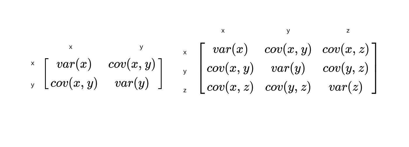
What is the 2 × 2 Covariance Matrix Formula?
The formula for a 2 × 2 covariance matrix is as follows:
Σ = [ Var(X) Cov(X, Y) Cov(Y, X) Var(Y) ]
Where Var(X) and Var(Y) represent the variances of variables X and Y, and Cov(X, Y) and Cov(Y, X) represent the covariances between variables X and Y.
What is the 3 × 3 Covariance Matrix Formula?
The formula for a 3 × 3 covariance matrix is as follows:
Σ = [ Var(X1) Cov(X1, X2) Cov(X1, X3) Cov(X2, X1) Var(X2) Cov(X2, X3) Cov(X3, X1) Cov(X3, X2) Var(X3) ]
Where Var(X1), Var(X2), and Var(X3) represent the variances of variables X1, X2, and X3, respectively, and Cov(X1, X2), Cov(X1, X3), and Cov(X2, X3) represent the covariances between pairs of variables.
Is the Variance Covariance Matrix Symmetric?
Yes, the variance-covariance matrix is always symmetric. This means that the element in the ith row and jth column is equal to the element in the jth row and ith column. The symmetry of the variance-covariance matrix arises from the symmetry of the covariances between variables.
Solved Examples on Covariance Matrix
Addition to Constant Vectors
Suppose we have a constant vector a = [3, 2, 1] and a random vector X = [X1, X2, X3] with covariance matrix Σ.
To find the covariance matrix of the new random vector Y = X + a, we can use the property that the covariance matrix remains unchanged when a constant vector is added to each observation.
The covariance matrix of Y is the same as the covariance matrix of X, which is Σ.
Multiplication by Constant Matrices
Suppose we have a constant matrix A = [2, 0, 1; 0, 3, 1; 1, 1, 2] and a random vector X = [X1, X2, X3] with covariance matrix Σ.
To find the covariance matrix of the new random vector Y = AX, we can use the property that the covariance matrix is transformed by the following rule:
Σ’ = AΣA^T
Where Σ’ is the transformed covariance matrix, Σ is the original covariance matrix, and A is the constant matrix.
By substituting the values into the formula, we can calculate the covariance matrix of Y.
Linear Transformations
Suppose we have a constant vector a = [2, 1] and a constant matrix A = [1, 0; 0, -1] and a random vector X = [X1, X2] with covariance matrix Σ.
To find the covariance matrix of the new random vector Y = AX + a, we can use the property of linear transformations of the covariance matrix:
Σ’ = AΣA^T
Where Σ’ is the transformed covariance matrix, Σ is the original covariance matrix, and A is the matrix representing the linear transformation.
By substituting the values into the formula, we can calculate the covariance matrix of Y.
These solved examples demonstrate how the covariance matrix is affected by addition to constant vectors, multiplication by constant matrices, and linear transformations. The covariance matrix provides valuable insights into the relationships and variability between variables in a dataset, allowing for further analysis and modeling.
How Kunduz Can Help You Learn Covariance Matrix?
At Kunduz, we understand the importance of mastering the concept of covariance matrix in statistical analysis and data modeling. That’s why we offer comprehensive learning resources, including tutorials, practice exercises, and interactive tools, to help you understand and apply the principles of covariance matrix effectively.
Our step-by-step tutorials provide clear explanations and examples of how to calculate and interpret covariance matrix. You can practice your skills with our interactive exercises, which offer real-world scenarios and datasets for hands-on learning. Our expert instructors are also available to provide guidance and answer any questions you may have along the way.
Whether you’re a beginner or an experienced data analyst, Kunduz is your trusted partner in mastering the concept of covariance matrix. Start your learning journey with us today and unlock the power of covariance matrix in statistical analysis and data modeling.
For readers delving into the intricacies of matrices, our matrix multiplication page serves as a valuable reference. It provides essential insights into the mathematical operations involved in multiplying matrices, offering a foundational understanding that contributes to a comprehensive grasp of covariance matrix computations.