State Alabama Alaska Arizona Arkansas California Colorado
Last updated: 9/7/2023
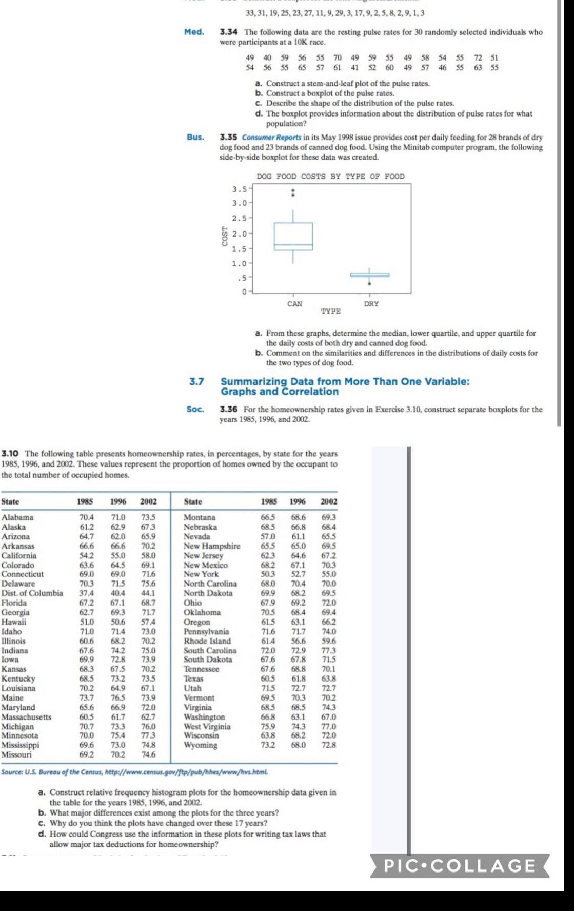
State Alabama Alaska Arizona Arkansas California Colorado Connecticut Delaware Dist of Columbia Florida Georgia Hawaii Idaho Illinois Indiana Iowa Med 1985 1996 2002 70 4 71 0 73 5 61 2 62 9 67 3 64 7 62 0 65 9 66 6 66 6 70 2 54 2 55 0 58 0 63 6 64 5 69 1 69 0 69 0 716 70 3 71 5 75 6 37 4 40 4 44 1 67 2 67 1 68 7 62 7 69 3 71 7 51 0 50 6 57 4 71 0 71 4 73 0 60 6 68 2 Bus 3 7 Soc State 33 31 19 25 23 27 11 9 29 3 17 9 2 5 8 2 9 1 3 3 34 The following data are the resting pulse rates for 30 randomly selected individuals who were participants at a 10K race Montana Nebraska Nevada COST 49 40 59 56 55 70 49 59 55 49 58 54 56 55 65 57 61 41 52 60 49 57 3 35 Consumer Reports in its May 1998 issue provides cost per daily feeding for 28 brands of dry dog food and 23 brands of canned dog food Using the Minitab computer program the following side by side boxplot for these data was created 3 5 3 0 2 5 2 0 1 5 1 0 5 0 a Construct a stem and leaf plot of the pulse rates b Construct a boxplot of the pulse rates c Describe the shape of the distribution of the pulse rates d The boxplot provides information about the distribution of pulse rates for what population DOG FOOD COSTS BY TYPE OF FOOD New Hampshire New Jersey New Mexico New York North Carolina North Dakota Ohio Oklahoma Oregon Pennsylvania Rhode Island South Carolina South Dakota Tennessee Texas Utah Vermont Virginia Washington West Virginia Wisconsin Wyoming 3 10 The following table presents homeownership rates in percentages by state for the years 1985 1996 and 2002 These values represent the proportion of homes owned by the occupant to the total number of occupied homes CAN TYPE a From these graphs determine the median lower quartile and upper quartile for the daily costs of both dry and canned dog food b Comment on the similarities and differences in the distributions of daily costs for the two types of dog food Summarizing Data from More Than One Variable Graphs and Correlation 70 2 67 6 74 2 75 0 69 9 72 8 73 9 68 3 67 5 70 2 Kansas Kentucky Louisiana Maine Maryland Massachusetts Michigan Minnesota Mississippi Missouri 68 5 73 2 73 5 70 2 64 9 67 1 73 7 76 5 73 9 65 6 66 9 72 0 60 5 61 7 62 7 70 7 73 3 76 0 70 0 75 4 77 3 69 6 73 0 74 8 69 2 70 2 74 6 Source U S Bureau of the Census http www census gov ftp pub hhes www hvs html 3 36 For the homeownership rates given in Exercise 3 10 construct separate boxplots for the years 1985 1996 and 2002 1985 66 5 68 6 68 5 66 8 57 0 61 1 65 5 65 0 62 3 64 6 68 2 67 1 70 3 50 3 68 0 52 7 55 0 70 4 70 0 69 5 69 9 68 2 67 9 69 2 72 0 69 4 70 5 68 4 61 5 63 1 66 2 56 6 59 6 71 6 71 7 74 0 61 4 72 0 72 9 77 3 67 6 67 8 71 5 67 6 68 8 70 1 60 5 61 8 63 8 71 5 72 7 72 7 69 5 70 2 70 3 68 5 74 3 68 5 66 8 63 1 67 0 75 9 74 3 77 0 63 8 68 2 72 0 73 2 68 0 72 8 b What major differences exist among the plots for the three years c Why do you think the plots have changed over these 17 years 1996 2002 69 3 68 4 54 55 72 51 46 55 63 55 DRY 65 5 69 5 67 2 a Construct relative frequency histogram plots for the homeownership data given in the table for the years 1985 1996 and 2002 d How could Congress use the information in these plots for writing tax laws that allow major tax deductions for homeownership PIC COLLAGE