
The Intermediate Value Theorem (IVT) is a fundamental concept in calculus that helps us understand the behavior of continuous functions. It provides insights into the existence of solutions and the range of values a function can take on within a given interval. In this comprehensive guide, we will explore the Intermediate Value Theorem in detail, including its statement, formula, proof, applications, and solved examples.
An Introduction to Intermediate Value Theorem
Calculus is a branch of mathematics that deals with the study of continuous change. One important concept in calculus is the Intermediate Value Theorem (IVT), which establishes a relationship between the continuity of a function and its range of values. The IVT is a powerful tool that allows us to analyze functions and make deductions about their behavior.
The IVT is closely related to the concept of continuity. A function is said to be continuous if it is defined for all points in its domain and has no abrupt jumps or breaks. In other words, a function is continuous if its graph can be drawn without lifting the pencil. The IVT provides a guarantee that a continuous function will take on every value between two given points.
What is the Intermediate Value Theorem?
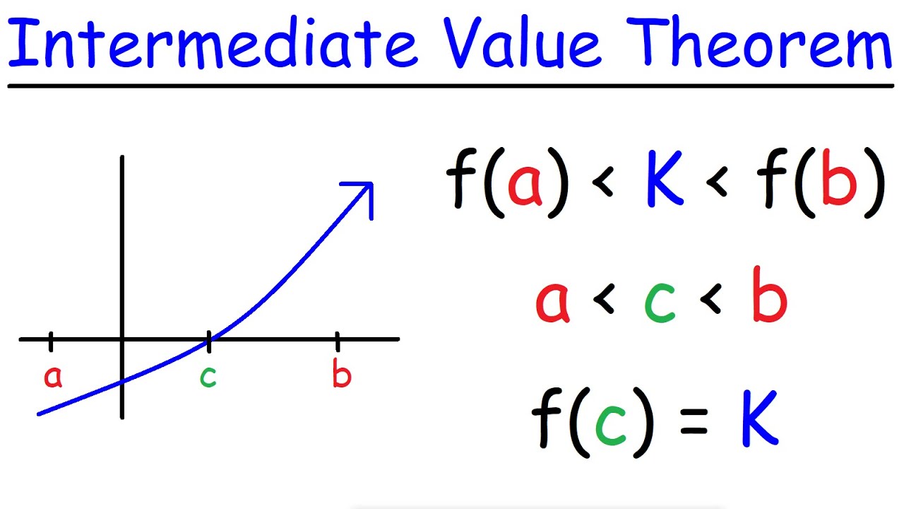
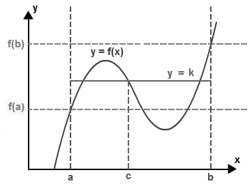
The Intermediate Value Theorem states that if a function f(x) is continuous over a closed interval [a, b], and L is any value between f(a) and f(b), then there exists at least one value c in the interval (a, b) such that f(c) = L. In simpler terms, if a function is continuous over an interval, it must take on every value between the function values at the endpoints of the interval.
This theorem is particularly useful when we want to verify the existence of a root (or a zero) of a function within a given interval. It helps us determine whether a function changes sign, and therefore has a root, between two points. The IVT can also be used to verify the existence of x-intercepts and to solve certain types of equations.
Intermediate Value Theorem Statement
The Intermediate Value Theorem can be stated as follows:
Intermediate Value Theorem: Suppose f(x) is a continuous function on a closed interval [a, b], and L is a value that lies between f(a) and f(b). Then, there exists at least one value c in the interval (a, b) such that f(c) = L.
In essence, the IVT guarantees that if a continuous function takes on two different values at the endpoints of an interval, it must also take on every value in between.
Intermediate Value Theorem Formula
The Intermediate Value Theorem is not defined by a specific formula, but rather by the concept of continuity. However, we can use the IVT to verify the existence of solutions to equations within a given interval.
Suppose we have a continuous function f(x) defined on the interval [a, b]. If we want to find a value c in the interval (a, b) such that f(c) = L, where L is a value between f(a) and f(b), we can use the Intermediate Value Theorem to determine whether such a value exists.
To apply the IVT, we need to follow these steps:
- Evaluate f(a) and f(b) to determine the function values at the endpoints of the interval.
- Check if L lies between f(a) and f(b). If L is not between f(a) and f(b), the IVT cannot be applied.
- If L is between f(a) and f(b), the IVT guarantees the existence of at least one value c in the interval (a, b) such that f(c) = L.
By using the Intermediate Value Theorem, we can establish the existence of solutions to equations within a given interval.
Intermediate Value Theorem Proof
The Intermediate Value Theorem can be proved using the concept of continuity and the least upper bound property of real numbers. The proof involves constructing a set of points that lie between the function values at the endpoints of the interval.
Let’s assume that f(x) is a continuous function on the closed interval [a, b] and L is a value that lies between f(a) and f(b). We can prove the existence of a value c in the interval (a, b) such that f(c) = L.
To prove this, we will consider the set A = { x ∈ [a, b]: f(x) < L }. We can show that this set is non-empty and bounded above by b. Therefore, it has a supremum, denoted as c.
By the continuity of f(x) at the endpoints a and b, we can prove that f(c) ≠ f(a) and f(c) ≠ f(b). This implies that c ∈ (a, b).
To establish f(c) = L, we need to prove both f(c) ≤ L and f(c) ≥ L.
The proof of f(c) ≤ L involves using the supremum property. We can construct a sequence xn ∈ A with xn → c. Since f(x) is continuous, f(xn) → f(c). Since xn ∈ A, we have f(xn) < L. Therefore, f(c) = limn → ∞ f(xn) ≤ L.
The proof of f(c) ≥ L involves considering a value tn = c + (1/n) for a very small n. Since tn > c, tn > supremum of A, which implies tn ∉ A. Thus, f(tn) ≥ L. Using the continuity of f(x), we have f(tn) → f(c). Therefore, f(c) = limn → ∞ f(tn) ≥ L.
From these proofs, we can conclude that f(c) = L, satisfying the Intermediate Value Theorem.
How To Use The Intermediate Value Theorem?
The Intermediate Value Theorem is a powerful tool in calculus that can be used to verify the existence of solutions to equations and to analyze the behavior of continuous functions. Here is a step-by-step guide on how to use the Intermediate Value Theorem effectively:
Step 1: Identify the function and the interval: Start by identifying the function for which you want to verify the existence of a solution or analyze its behavior. Determine the interval over which you want to apply the Intermediate Value Theorem.
Step 2: Evaluate the function values at the endpoints: Calculate the function values at the endpoints of the interval. This will give you f(a) and f(b), where a and b are the endpoints of the interval.
Step 3: Check if the function values bracket the desired value: Determine whether the desired value, let’s say L, lies between f(a) and f(b). If L is not between f(a) and f(b), the Intermediate Value Theorem cannot be applied.
Step 4: Apply the Intermediate Value Theorem: If L lies between f(a) and f(b), the Intermediate Value Theorem guarantees the existence of at least one value c in the interval (a, b) such that f(c) = L. This means that the function must cross the line y = L at some point within the interval.
Step 5: Solve for the value of c: Use numerical methods or algebraic techniques to find the value of c that satisfies f(c) = L. This may involve solving equations or using approximation methods such as bisection or Newton’s method.
Step 6: Verify the solution: Once you have found the value of c, substitute it back into the original function to verify that f(c) = L. This step ensures that the solution obtained is accurate.
By following these steps, you can effectively utilize the Intermediate Value Theorem to analyze functions and verify the existence of solutions within a given interval.
Continuous Functions and Intermediate Value Theorem
The Intermediate Value Theorem is closely related to the concept of continuity. A function is said to be continuous if it is defined for all points in its domain and has no abrupt jumps or breaks. In other words, a function is continuous if its graph can be drawn without lifting the pencil.
For the Intermediate Value Theorem to hold, the function must be continuous over the closed interval [a, b]. This means that the function does not have any sudden changes or discontinuities within the interval. Continuity ensures that the function can take on every value between f(a) and f(b).
Continuous functions are essential in calculus because they allow us to make precise calculations and draw meaningful conclusions about the behavior of functions. The Intermediate Value Theorem is a powerful tool that relies on the continuity of a function to establish the existence of solutions and the range of values a function can take on within a given interval.
Intermediate Value Theorem vs. Mean Value Theorem
The Intermediate Value Theorem and the Mean Value Theorem are both fundamental concepts in calculus that deal with the behavior of functions. While they share some similarities, they have distinct differences in their statements and applications.
The Intermediate Value Theorem guarantees the existence of a value within an interval where a function takes on a specific value. It establishes that if a function is continuous over a closed interval [a, b], it must take on every value between f(a) and f(b). This theorem is particularly useful for verifying the existence of solutions to equations and analyzing the behavior of functions.
On the other hand, the Mean Value Theorem states that if a function is continuous over a closed interval [a, b] and differentiable over the open interval (a, b), then there exists at least one value c in the interval (a, b) such that the instantaneous rate of change (slope) of the function at c is equal to the average rate of change of the function over the interval [a, b]. The Mean Value Theorem is often used to prove important results in calculus, such as the relationship between the derivative and the integral.
While both the Intermediate Value Theorem and the Mean Value Theorem are powerful tools in calculus, they serve different purposes. The Intermediate Value Theorem focuses on the existence of values within an interval, while the Mean Value Theorem relates the derivative and the average rate of change of a function.
Intermediate Value Theorem Applications
The Intermediate Value Theorem has various applications in calculus and real-world problem-solving. Some of the key applications of the Intermediate Value Theorem are:
- Existence of Solutions: The IVT can be used to verify the existence of solutions to equations within a given interval. By checking if the function values at the endpoints of the interval have different signs, we can conclude that the function has at least one root (or zero) within the interval.
- Verification of x-intercepts: The IVT can be used to verify the existence of x-intercepts (or zeros) of a function within a given interval. If the function values at the endpoints have different signs, we can conclude that the function has at least one x-intercept within the interval.
- Bisection Method: The IVT is often employed in numerical methods, such as the bisection method, to approximate the roots of an equation. By dividing the interval into smaller subintervals and applying the IVT, we can find an interval that contains the root.
- Analysis of Function Behavior: The IVT allows us to analyze the behavior of functions by determining if they change sign or take on specific values within a given interval. This information is crucial for understanding the properties and characteristics of functions.
- Existence of Solutions to Differential Equations: The IVT can be used to establish the existence of solutions to certain types of differential equations. By applying the IVT to specific intervals, we can determine if a solution exists within that interval.
These are just a few examples of how the Intermediate Value Theorem is applied in calculus and problem-solving. The IVT provides a powerful tool for analyzing functions and establishing the existence of solutions within a given interval.
Solved Examples on Intermediate Value Theorem
Let’s now explore some solved examples to understand how the Intermediate Value Theorem is applied in practice.
Example 1: Verify if the function f(x) = x^2 – 3x + 2 has a root in the interval [1, 3].
Solution: To determine if the function has a root in the interval [1, 3], we need to evaluate f(1) and f(3).
f(1) = 1^2 – 3(1) + 2 = 0 f(3) = 3^2 – 3(3) + 2 = 2
Since f(1) = 0 and f(3) = 2 have different signs (one is positive, the other is negative), we can conclude that the function has a root within the interval [1, 3] according to the Intermediate Value Theorem.
Example 2: Determine if the equation cos(x) = x has a solution in the interval [0, 1].
Solution: To determine if the equation has a solution in the interval [0, 1], we need to evaluate cos(0) and cos(1).
cos(0) = 1 cos(1) ≈ 0.5403
Since cos(0) = 1 and cos(1) ≈ 0.5403 have different signs, we can conclude that the equation cos(x) = x has a solution within the interval [0, 1] according to the Intermediate Value Theorem.
These examples demonstrate how the Intermediate Value Theorem can be applied to verify the existence of solutions within a given interval. By evaluating the function values at the endpoints and checking if they have different signs, we can determine if a function has a root or a solution within the interval.
Frequently Asked Questions on Intermediate Value Theorem
Q1. What is the Intermediate Value Theorem?
The Intermediate Value Theorem is a key principle in calculus that states if a function is continuous on an interval [a, b], then for every y-value between f(a) and f(b), there exists some x-value in the interval (a, b).
Q2. How do you apply the Intermediate Value Theorem?
To apply the Intermediate Value Theorem, you first need to ensure that the function is continuous on the given interval. Then, identify a value that lies between the function values at the endpoints of the interval. If such a value exists, the Intermediate Value Theorem guarantees that there is a point within the interval where the function takes on this value.
Q3. What are the requirements for the Intermediate Value Theorem?
The Intermediate Value Theorem requires a function to be continuous on a closed interval [a, b]. Additionally, a number N must exist such that N lies between f(a) and f(b), where f(a) ≠ f(b).
Q4. How is the Intermediate Value Theorem used in calculus?
In calculus, the Intermediate Value Theorem is primarily used to verify whether an equation has a solution within a specified interval. It provides a theoretical foundation to confirm that a solution exists, without necessarily finding the exact value of the solution.
Q5. What is the difference between the Intermediate Value Theorem and the Mean Value Theorem?
While both the Intermediate Value Theorem and the Mean Value Theorem are fundamental principles in calculus, they serve different purposes. The Intermediate Value Theorem deals with the existence of solutions within a specific interval for a continuous function. In contrast, the Mean Value Theorem relates the average rate of change of a function over an interval to the instantaneous rate of change at a specific point within the interval.
How Kunduz Can Help You Learn Intermediate Value Theorem?
At Kunduz, we understand the challenges students face when learning calculus and the Intermediate Value Theorem. That’s why we have developed comprehensive courses and resources to help you master this important concept.
Our courses are designed by experienced mathematicians and teachers who have a deep understanding of the Intermediate Value Theorem and its applications. With personalized attention from our expert tutors, you can gain a solid understanding of the Intermediate Value Theorem and excel in your calculus studies.