
Binomial distribution is a probability distribution that models the number of successes in a fixed number of independent Bernoulli trials. It is a discrete distribution, meaning that the possible outcomes are countable and distinct. The binomial distribution is widely used in statistics, finance, and quality control, among other fields.
What is Binomial Distribution?
Binomial distribution is a probability distribution that describes the number of successes in a fixed number of independent Bernoulli trials. Each trial has two possible outcomes, usually referred to as success and failure. The probability of success in each trial is denoted by “p,” while the probability of failure is denoted by “q” (where q = 1 – p). The parameters of the binomial distribution are the number of trials, denoted by “n,” and the probability of success, denoted by “p.”

Binomial Distribution Formula
The formula for the binomial distribution is:
P(X = k) = nCk * p^k * (1-p)^(n-k)
where:
- P(X = k) is the probability of getting exactly k successes in n trials,
- nCk is the number of combinations of n things taken k at a time,
- p is the probability of success in a single trial, and
- (1-p) is the probability of failure in a single trial.
The binomial distribution formula calculates the probability of obtaining a specific number of successes, k, in a fixed number of trials, n.
Binomial Distribution Calculation
To calculate the probability of a specific number of successes in a binomial distribution, you need to plug in the values of n, k, p, and (1-p) into the binomial distribution formula. The number of combinations, nCk, can be calculated using the formula:
nCk = n! / (k! * (n-k)!)
where “!” denotes the factorial function.
Once you have calculated nCk, you can substitute all the values into the binomial distribution formula to obtain the probability.
Binomial Probability Distribution
The binomial probability distribution is a table or graph that shows the probabilities of obtaining each possible number of successes in a binomial distribution. It provides a visual representation of the probabilities associated with different values of k in the binomial distribution.
The binomial probability distribution can be calculated using the binomial distribution formula for each value of k. The probabilities for all possible values of k should sum up to 1.
How To Find Binomial Probability?
To find the binomial probability, you need to follow these steps:
- Identify the values of n, k, p, and (1-p) in the binomial distribution problem.
- Calculate the number of combinations, nCk, using the formula n! / (k! * (n-k)!).
- Substitute the values of nCk, p, and (1-p) into the binomial distribution formula: P(X = k) = nCk * p^k * (1-p)^(n-k).
- Calculate the probability using the formula.
- Repeat steps 2-4 for each value of k to obtain the complete binomial probability distribution.
Negative Binomial Distribution
The negative binomial distribution is a generalization of the binomial distribution that models the number of failures that occur before a specified number of successes in a series of independent Bernoulli trials. It is used when the trials continue until a certain number of successes are achieved.
Binomial Distribution Mean and Variance
The mean and variance of a binomial distribution can be calculated using the following formulas:
Mean (μ) = n * p Variance (σ^2) = n * p * (1 – p)
where:
- n is the number of trials,
- p is the probability of success in a single trial,
- μ is the mean, and
- σ^2 is the variance.
The mean represents the average number of successes in the binomial distribution, while the variance measures the spread or dispersion of the distribution.
Binomial Distribution Vs Normal Distribution
The main difference between the binomial distribution and the normal distribution is that the binomial distribution is discrete, while the normal distribution is continuous. The binomial distribution describes the number of successes in a fixed number of independent trials with two possible outcomes. The normal distribution, on the other hand, describes continuous random variables and is widely used to approximate various phenomena in nature.
While the binomial distribution is appropriate for discrete data and a small number of trials, the normal distribution is suitable for continuous data and large sample sizes. As the number of trials in a binomial distribution increases, the distribution becomes more symmetric and bell-shaped, resembling the normal distribution.
Properties of Binomial Distribution
The binomial distribution has several important properties:
- There are only two possible outcomes: success or failure, yes or no, true or false.
- The number of trials is fixed and denoted by “n.”
- The probability of success in each trial is constant and denoted by “p.”
- The number of successes is calculated out of all trials.
- Each trial is independent of any other trial.
These properties make the binomial distribution a versatile tool for modeling real-world phenomena and conducting statistical analyses.
Probability Mass Function
The probability mass function (PMF) is a function that describes the probabilities of obtaining each possible value in a discrete probability distribution. For the binomial distribution, the PMF gives the probability of obtaining each possible number of successes in a fixed number of trials.
The PMF of the binomial distribution is given by the binomial distribution formula:
P(X = k) = nCk * p^k * (1-p)^(n-k)
where P(X = k) is the probability of obtaining exactly k successes in n trials, nCk is the number of combinations, p is the probability of success in a single trial, and (1-p) is the probability of failure in a single trial.
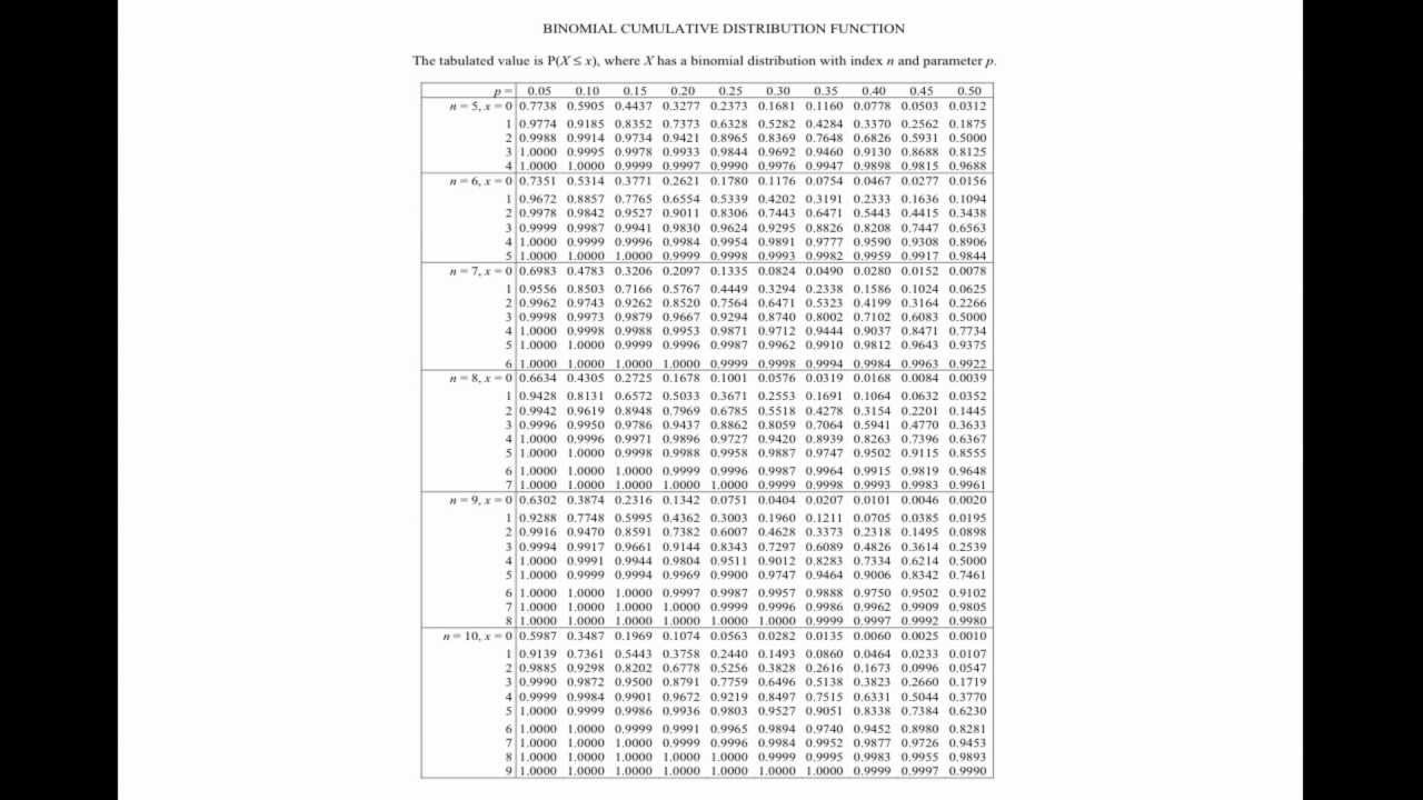
Cumulative Distribution Function
The cumulative distribution function (CDF) is a function that gives the probability that a random variable is less than or equal to a specified value. For the binomial distribution, the CDF gives the probability of obtaining up to a certain number of successes in a fixed number of trials.
The CDF of the binomial distribution can be calculated by summing the probabilities of obtaining each possible number of successes up to the desired value. This can be done using the binomial distribution formula for each value of k and summing the probabilities.
Related Distributions
The binomial distribution is related to several other probability distributions, including:
- Sums of binomials: The sum of two or more independent binomial random variables is also a binomial random variable.
- Poisson binomial distribution: The distribution of the number of successes in a sequence of independent and non-identically distributed Bernoulli trials.
- Ratio of two binomial distributions: The ratio of two independent binomial random variables follows a specific distribution.
- Conditional binomials: The distribution of the number of successes in a sequence of independent Bernoulli trials, given that a certain number of failures has already occurred.
- Bernoulli distribution: The binomial distribution is a generalization of the Bernoulli distribution, which models a single trial with two possible outcomes.
- Normal approximation: The binomial distribution can be approximated by the normal distribution under certain conditions.
- Poisson approximation: The binomial distribution can be approximated by the Poisson distribution when the number of trials is large and the success probability is small.
- Limiting distributions: The binomial distribution approaches the normal distribution as the number of trials becomes large.
Standard Deviation of the Binomial Distribution
The standard deviation of the binomial distribution measures the variability or dispersion of the distribution. It can be calculated using the following formula:
Standard Deviation (σ) = sqrt(n * p * (1 – p))
where:
- n is the number of trials,
- p is the probability of success in a single trial, and
- sqrt denotes the square root function.
The standard deviation represents the spread of the binomial distribution. It indicates how much the values of the random variable deviate from the mean.
Bernoulli Trial
A Bernoulli trial is a random experiment with two possible outcomes: success and failure. It is a special case of a binomial trial, where there is only one trial. The outcomes of a Bernoulli trial are usually denoted as 1 for success and 0 for failure.
The binomial distribution is a generalization of the Bernoulli distribution to multiple trials. Each trial in a binomial distribution is a Bernoulli trial.
Binomial Distribution Table
A binomial distribution table is a tabular representation of the probabilities associated with different numbers of successes in a binomial distribution. It provides an easy way to look up the probabilities for specific values of k.
The table typically includes the values of k, the corresponding probabilities, and the cumulative probabilities. The cumulative probabilities show the probability of obtaining up to a certain number of successes.
Binomial distribution tables can be used to quickly find the probabilities for specific values of k without performing calculations using the binomial distribution formula.
Binomial Distribution Graph
A binomial distribution graph is a visual representation of the probabilities associated with different numbers of successes in a binomial distribution. It provides a way to visualize the distribution and understand its shape.
In a binomial distribution graph, the x-axis represents the number of successes, and the y-axis represents the probability. The graph typically shows bars or points for each value of k, with the height of each bar or point indicating the probability.
The binomial distribution graph is useful for understanding the probabilities associated with different values of k and identifying patterns or trends in the distribution.

Measure of Central Tendency for Binomial Distribution
The measure of central tendency for a binomial distribution is the value that represents the center or average of the distribution. It provides a summary of the typical or expected value of the random variable.
The mean, or expected value, is the measure of central tendency for a binomial distribution. It represents the average number of successes in the distribution. The mean can be calculated using the formula:
Mean (μ) = n * p
where:
- μ is the mean,
- n is the number of trials, and
- p is the probability of success in a single trial.
The mean is a useful summary statistic for understanding the center of the distribution and making comparisons between different binomial distributions.
Solved Examples on Binomial Distribution
Let’s work through some examples to illustrate how to apply the binomial distribution formula and calculate probabilities in real-world scenarios.
Example 1: A fair coin is flipped 10 times. What is the probability of getting exactly 5 heads?
Solution: In this example, n = 10 (number of trials), k = 5 (number of successes), and p = 0.5 (probability of success in a single trial). We can calculate the probability using the binomial distribution formula:
P(X = 5) = 10C5 * (0.5)^5 * (1-0.5)^(10-5)
Using the combination formula, 10C5 = 10! / (5! * (10-5)!), we can find the value of 10C5. Plugging in the values, we have:
P(X = 5) = 252 * (0.5)^5 * (0.5)^5
P(X = 5) = 252 * 0.03125 * 0.03125
P(X = 5) = 0.0778
Therefore, the probability of getting exactly 5 heads in 10 coin flips is approximately 0.0778.
Example 2: A manufacturing process produces defective items with a probability of 0.1. If 100 items are produced, what is the probability of having at least 10 defective items?
Solution: In this example, n = 100 (number of trials), k is the number of defective items, and p = 0.1 (probability of producing a defective item). We want to calculate the probability of having at least 10 defective items, which is equivalent to finding the probability of having 10, 11, 12, …, 100 defective items and summing them.
P(X ≥ 10) = P(X = 10) + P(X = 11) + … + P(X = 100)
Using the binomial distribution formula, we can calculate each individual probability and sum them up.
P(X = k) = 100Ck * (0.1)^k * (1-0.1)^(100-k)
Plugging in the values, we have:
P(X = 10) = 100C10 * (0.1)^10 * (1-0.1)^(100-10) P(X = 11) = 100C11 * (0.1)^11 * (1-0.1)^(100-11) … P(X = 100) = 100C100 * (0.1)^100 * (1-0.1)^(100-100)
Calculate each individual probability using the combination formula, and then sum them up to find P(X ≥ 10).
By solving these examples, we can see how the binomial distribution formula can be used to calculate probabilities in various scenarios.
How Kunduz Can Help You Learn Binomial Distribution?
Kunduz is an online learning platform that provides comprehensive resources to help you learn and understand binomial distribution. Through interactive lessons, video tutorials, and practice problems, Kunduz offers a structured and engaging learning experience.
With Kunduz, you can:
- Learn the concepts and principles of binomial distribution from expert instructors.
- Gain a deep understanding of the binomial distribution formula and its applications.
- Practice solving a wide range of binomial distribution problems to strengthen your skills.
- Access additional resources, such as worksheets and quizzes, to reinforce your learning.
Whether you’re a student studying statistics or a professional looking to enhance your data analysis skills, Kunduz can help you master binomial distribution and apply it effectively in real-world scenarios. Experience the convenience and effectiveness of online learning with Kunduz today!