Algebra Questions
The best high school and college tutors are just a click away, 24×7! Pick a subject, ask a question, and get a detailed, handwritten solution personalized for you in minutes. We cover Math, Physics, Chemistry & Biology.
Algebra
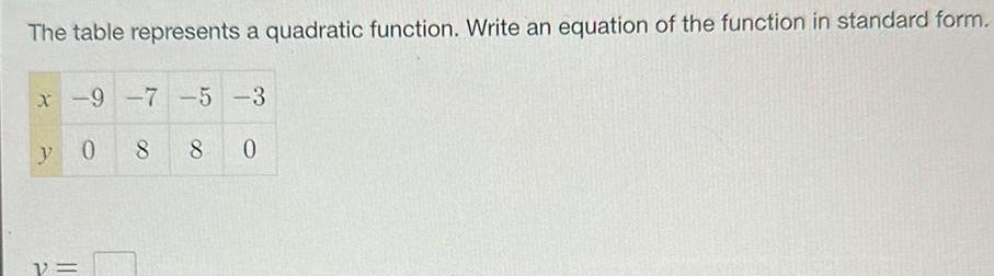
Quadratic equationsThe table represents a quadratic function Write an equation of the function in standard form x 9 7 5 3 8 y 0 2 8 0
Algebra
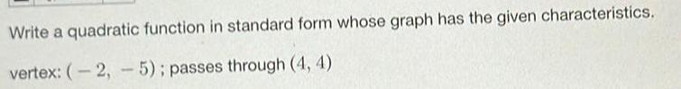
Quadratic equationsWrite a quadratic function in standard form whose graph has the given characteristics vertex 2 5 passes through 4 4
Algebra
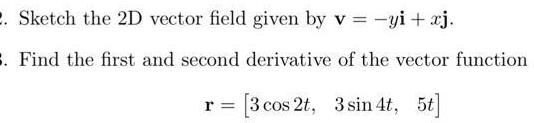
Complex numbersSketch the 2D vector field given by v yi xj 3 Find the first and second derivative of the vector function r 3 cos 2t 3 sin 4t 5t
Algebra
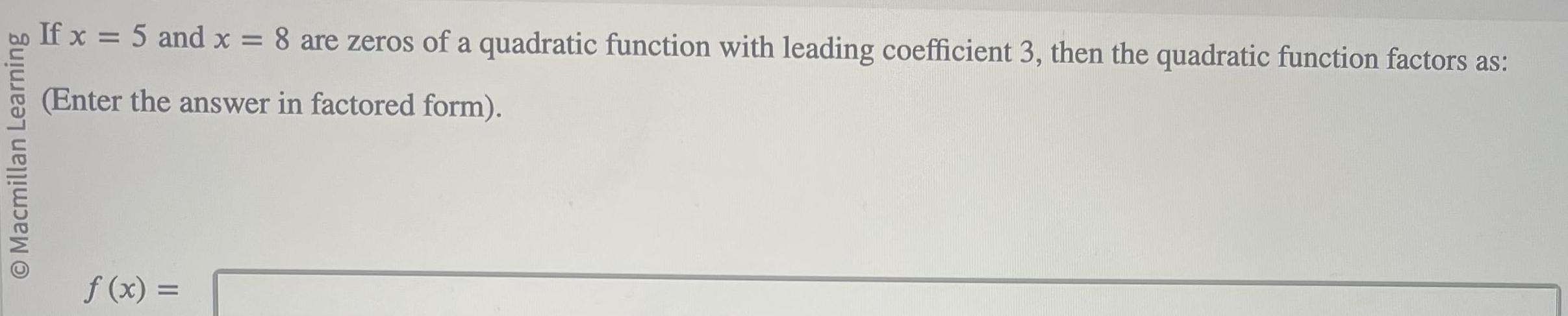
Quadratic equationsO Macmillan Learning If x 5 and x 8 are zeros of a quadratic function with leading coefficient 3 then the quadratic function factors as Enter the answer in factored form f x
Algebra
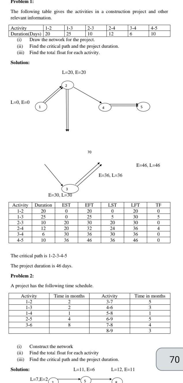
Sequences & SeriesProblem 1 The following table gives the activities in a construction project and other relevant information Activity 1 2 1 3 2 3 Duration Days 20 25 10 i Draw the network for the project ii Find the critical path and the project duration iii Find the total float for each activity Solution L 0 E 0 Activity 1 2 1 3 2 3 2 4 3 4 4 5 1 i ii iii Solution 3 E 30 L 30 Duration 20 25 10 12 6 10 L 20 E 20 EST 0 0 L 7 E 26 20 20 30 36 The critical path is 1 2 3 4 5 The project duration is 46 days Problem 2 A project has the following time schedule Time in months Activity 1 2 2 1 3 2 1 4 1 2 5 3 6 4 8 70 EFT 20 25 30 32 36 46 5 2 4 12 E 36 L 36 LST 0 5 20 24 30 36 Activity 3 7 4 6 Construct the network Find the total float for each activity Find the critical path and the project duration L 11 E 6 5 8 6 9 7 8 8 9 3 4 6 LFT 20 30 30 36 36 46 5 E 46 L 46 L 12 E 11 4 5 10 TF 0 5 0 4 0 0 Time in months 5 3 1 5 4 3 70
Algebra
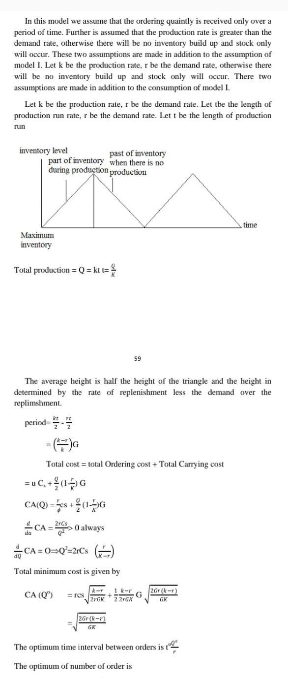
Sequences & SeriesIn this model we assume that the ordering quaintly is received only over a period of time Further is assumed that the production rate is greater than the demand rate otherwise there will be no inventory build up and stock only will occur These two assumptions are made in addition to the assumption of model I Let k be the production rate r be the demand rate otherwise there will be no inventory build up and stock only will occur There two assumptions are made in addition to the consumption of model I Let k be the production rate r be the demand rate Let tbe the length of production run rate r be the demand rate Let t be the length of production run inventory level past of inventory part of inventory when there is no during production production Maximum inventory Total production Q kt t period 1 The average height is half the height of the triangle and the height in determined by the rate of replenishment less the demand over the replimshment G Total cost total Ordering cost Total Carrying cost uC 1 G CA Q cs 1 G CA 2r 0 always CA O Q 2rCs Total minimum cost is given by 59 CA Q rcs k r 1 k r G 2rGK 2 2rGK 2Gr k r GK 2Gr k r GK time The optimum time interval between orders is t The optimum of number of order is

Algebra
Matrices & Determinantsn s 1 p sp n E 0 1 p s p 1 Sp N s 1 p 1 This queueing modrl with limited waiting room is valuable because of its relevance to many real situations and the fact that changes may be made to its properties by adjusting the number of servers or the capacity of the waiting room However while poission arrivals are common in practice negative exponential service times are less so and it is the second assumption in the system MIMs that limits its usefulness Example A supermarket has two girls ringing up stales at the counters If the service time for each customer is exponential with mean 4 minutes and if people arrive in a poission fashion at the counter at the rate of 10 per hour then calculate Solution a The probability of having to wait for service b The expected percentage of idle time for each girl c If a customer has to wait find the expected length of his waiting time a Probability of having to wait for service is P W 0 Po s 1 p 1 6 s s 2 Now compute Po 1 n 0 52 16 0 5 p s sp n sp s n n s 1 P n 0 2 1 3 2 1 3 1 2 3 4 9 2x2 31 1 2 Thusprob W 0 21 1 3 1 6 b The fraction of the time the service remains busy is given by p us 1 3 2 1 3 1 3 Theefore the fraction of the time thee service remains idle is 1 1 3 2 3 67 nearly c W W 0 3 minutes

Algebra
Matrices & DeterminantsThe following table gives the activities in a construction project and other relevant information Activity Duration Days i ii iii Solution L 0 E 0 Activity 1 2 1 3 2 3 20 25 10 Draw the network for the project 3 4 4 5 Duration 20 0 1 3 25 0 III 2 3 10 20 2 4 12 20 6 30 10 Find the critical path and the project duration Find the total float for each activity 1 2 Activity 1 2 1 3 1 4 2 5 3 6 L 20 E 20 3 E 30 L 30 The critical path is 1 2 3 4 5 The project duration is 46 days Solution T EST 36 Problem 2 A project has the following time schedule Time in months 2 2 1 4 8 75 20 70 EFT 20 25 30 32 36 46 i Construct the network ii Find the total float for each activity iii 2 4 12 E 36 L 36 LST 0 5 20 24 30 36 Find the critical path and the project duration L 11 E 6 Activity 3 7 4 6 5 8 6 9 7 8 8 9 3 4 6 LFT 20 30 30 36 36 46 5 E 46 L 46 L 12 E 11 4 5 10 TF 0 5 0 4 0 0 Time in months 5 3 1 5 4 3 70

Algebra
Matrices & DeterminantsNANA t The total cost per year C Q G Cs QC D GO Differenhating w r to Q We get dQ t d CA Q 2D doz Total ordering cost total inventory carrying cost C s C Gis always posture Q 0 is given by Q 2DG C For this value of Q CA Q in minimum toQus Q dQ 2DG 55 2DG C CA O 2DG When Q G This ordering quantity is denoted by Q t 56 time
Algebra
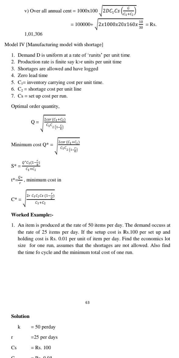
Permutations and CombinationsModel IV Manufacturing model with shortage 1 Demand D is uniform at a rate of runits per unit time 2 Production rate is finite say kor units per unit time 3 Shortages are allowed and have logged 4 Zero lead time 5 C inventory carrying cost per unit time 6 C shortage cost per unit line 7 Cs set up cost per run Optimal order quantity S v Over all annual cent 1000x100 2DC Cs C 1 01 306 Minimum cost Q Q G 1 G C t minimum cost in r Cs Q Solution k 2csr C C C 1 F 2r C C Cs 1 7 C C Worked Example 1 An item is produced at the rate of 50 items per day The demand occuss at the rate of 25 items per day If the setup cost is Rs 100 per set up and holding cost is Rs 0 01 per unit of item per day Find the economics lot size for one run assumes that the shortages are not allowed Also find the time fo cycle and the minimum total cost of one run 100000 2x1000x20x160x Rs 2 csr C C C C 1 1 50 perday 25 per days Rs 100 D 001 63
Algebra
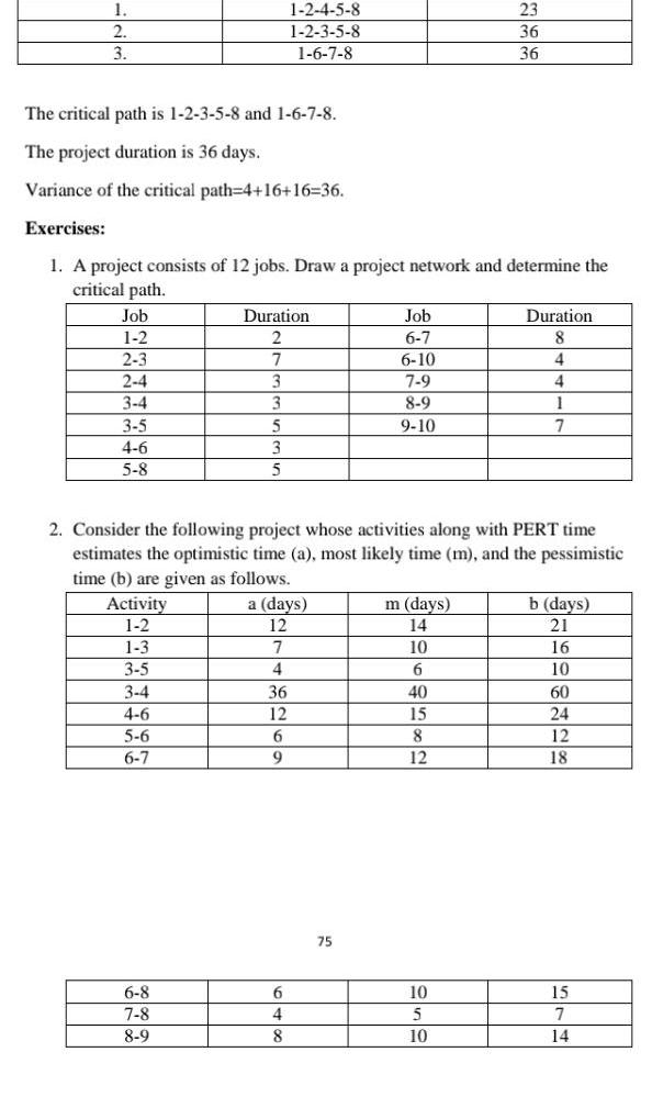
Quadratic equations1 2 3 The critical path is 1 2 3 5 8 and 1 6 7 8 The project duration is 36 days Variance of the critical path 4 16 16 36 Exercises 1 A project consists of 12 jobs Draw a project network and determine the critical path Job 1 2 2 3 2 4 3 4 3 5 4 6 5 8 Activity 1 2 1 3 3 5 3 4 4 6 5 6 6 7 1 2 4 5 8 1 2 3 5 8 1 6 7 8 6 8 7 8 8 9 Duration 2 7 3 3 5 3 5 2 Consider the following project whose activities along with PERT time estimates the optimistic time a most likely time m and the pessimistic time b are given as follows a days 12 7 4 36 12 6 9 6 4 8 Job 6 7 6 10 7 9 8 9 9 10 75 23 36 36 m days 14 10 6 40 15 8 12 10 5 10 Duration 8 4 4 1 7 b days 21 16 10 60 24 12 18 15 7 14

Algebra
Matrices & DeterminantsSolution Job 1 2 7 8 2 3 3 5 5 8 6 7 4 5 2 4 1 6 The various paths are 1 2 1 6 2 3 2 4 TE 1 2 3 3 5 4 5 6 7 5 8 7 8 3 TD Tp 4Tm The critical path is 1 2 3 5 8 The project duration is 36 days Variance of the critical path 4 16 4 1 25 6 42 6 7 108 6 18 84 6 14 66 6 11 24 6 4 66 6 11 42 6 7 30 6 5 36 6 6 3 2 6 2 5 3 1 2 3 5 8 1 2 4 5 8 1 6 7 8 3 1 4 73 5 SD Tp 2 4 4 2 1 4 2 1 2 6 Problem 4 The following table lists the jobs of a network with their time estimates Job Optimistic Duration days Most Likely 6 5 7 12 5 11 6 9 4 19 To Variance 16 16 4 1 16 4 1 4 Duration 36 23 35 Pessimistic HHGBHS 15 14 30 17 15 27 7 28 72
Algebra
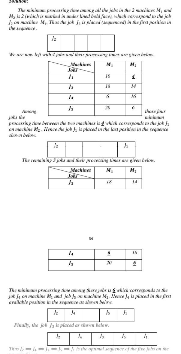
Sequences & SeriesSolution The minimum processing time among all the jobs in the 2 machines M and M is 2 which is marked in under lined bold face which correspond to the job J2 on machine M Thus the job J2 is placed sequenced in the first position in the sequence J2 We are now left with 4 jobs and their processing times are given below Machines M M Jobs J J3 J4 Js J2 Jobs J3 10 J4 Js 18 34 6 20 Among jobs the those four minimum processing time between the two machines is 4 which corresponds to the job J1 on machine M Hence the job J is placed in the last position in the sequence shown below The remaining 3 jobs and their processing times are given below Machines M M 18 J 6 20 14 16 6 J 14 16 6 The minimum processing time among these jobs is 6 which corresponds to the job J4 on machine M and job Js on machine M Hence J4 is placed in the first available position in the sequence as shown below Jz J4 J5 Finally the job J3 is placed as shown below J J4 J3 J5 J Thus J2J4J3 J5 J is the optimal sequence of the five jobs on the
Algebra
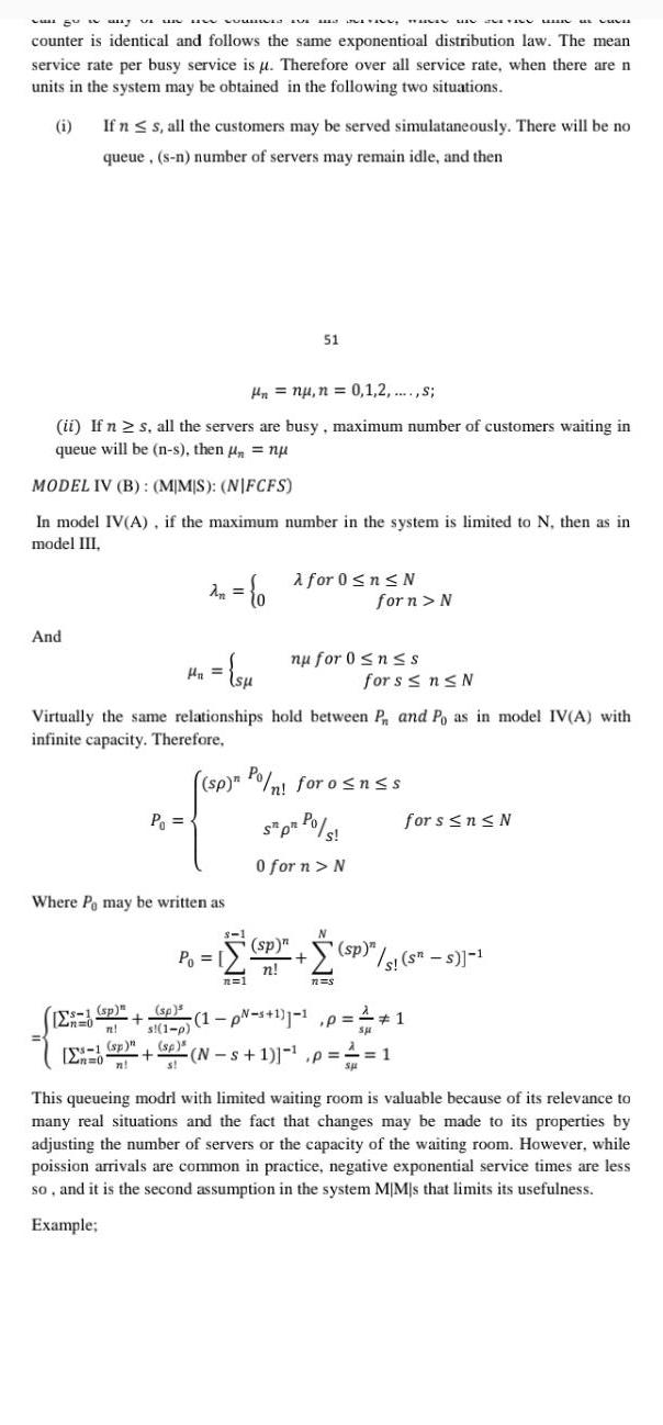
Sequences & Seriesagus any vi u uw won TAN counter is identical and follows the same exponentioal distribution law The mean service rate per busy service is u Therefore over all service rate when there are n units in the system may be obtained in the following two situations i And If n s all the customers may be served simulataneously There will be no queue s n number of servers may remain idle and then Hn nu n 0 1 2 s ii If n s all the servers are busy maximum number of customers waiting in queue will be n s then nu MODEL IV B MMS NIFCFS In model IV A if the maximum number in the system is limited to N then as in model III s 1 sp 12n 0 n sp Zn 0 n P An 0 H x su Where Pe may be written as sp s 1 p Virtually the same relationships hold between P and Po as in model IV A with infinite capacity Therefore 8 1 P 51 n 1 sp n Po nl foro nss St pt Po s s 0 for n N for 0 n N sp n n nu for 0 nss TUSIN MINU n s for n N 1 p s 1 1 1 p for s n N sp N s 1 p s sp sp s s s SH DUVA for s n N 1 1 This queueing modrl with limited waiting room is valuable because of its relevance to many real situations and the fact that changes may be made to its properties by adjusting the number of servers or the capacity of the waiting room However while poission arrivals are common in practice negative exponential service times are less so and it is the second assumption in the system MIM s that limits its usefulness Example

Algebra
Complex numbersShow that the equation sin sin is not an identity Which of the following values for can be used to show that the equation sin B sin B is NOT an identity A T 2 OC I B 2x OD O

Algebra
Complex numbersConsider the following function g t 4t 0 Use the Leading Coefficient Test to determine the end behavior of g The graph of g Select an answer to the left and Select an answer to the right 4
Algebra
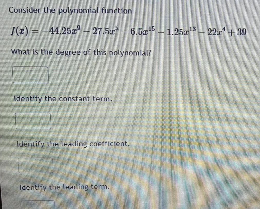
Quadratic equationsConsider the polynomial function f x 44 25x 27 5x5 6 5x 5 1 25x 3 22x 39 What is the degree of this polynomial Identify the constant term Identify the leading coefficient Identify the leading term

Algebra
Complex numbersConsider the polynomial function T 16 f x 6x 11c What is the degree of this polynomial Identify the constant term 12T Identify the leading coefficient Identify the leading term 14
Algebra
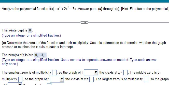
Quadratic equationsAnalyze the polynomial function f x x 2x 3x Answer parts a through e Hint First factor the polynomial The y intercept is 0 Type an integer or a simplified fraction c Determine the zeros of the function and their multiplicity Use this information to determine whether the graph crosses or touches the x axis at each x intercept The zero s of f is are 0 3 1 Type an integer or a simplified fraction Use a comma to separate answers as needed Type each answer only once The smallest zero is of multiplicity multiplicity so the graph of f so the graph of f the x axis at x The middle zero is of the x axis at x The largest zero is of multiplicity so the graph
Algebra
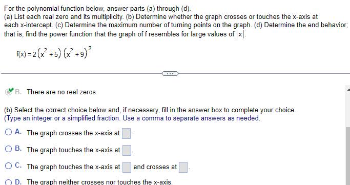
Quadratic equationsFor the polynomial function below answer parts a through d a List each real zero and its multiplicity b Determine whether the graph crosses or touches the x axis at each x intercept c Determine the maximum number of turning points on the graph d Determine the end behavior that is find the power function that the graph of f resembles for large values of x f x 2 x 5 x 9 B There are no real zeros b Select the correct choice below and if necessary fill in the answer box to complete your choice Type an integer or a simplified fraction Use comma to separate answer as needed OA The graph crosses the x axis at B The graph touches the x axis at OC The graph touches the x axis at and crosses at OD The graph neither crosses nor touches the x axis
Algebra
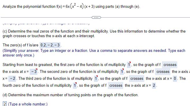
Quadratic equationsAnalyze the polynomial function f x 6x x 4 x 3 using parts a through e c Determine the real zeros of the function and their multiplicity Use this information to determine whether the graph crosses or touches the x axis at each x intercept The zero s off is are 0 2 2 3 Simplify your answer Type an integer or a fraction Use a comma to separate answers as needed Type each answer only once Starting from least to greatest the first zero of the function is of multiplicity 1 so the graph of f crosses the x axis at x 3 The second zero of the function is of multiplicity 1 so the graph of f crosses the x axis x 2 The third zero of the function is of multiplicity 1 so the graph of f crosses the x axis at x 0 The fourth zero of the function is of multiplicity 1 so the graph of f crosses the x axis at x 2 d Determine the maximum number of turning points on the graph of the function 2 Type a whole number

Algebra
Complex numbersUse transformations of the graph of y x to graph the function h x 2 x 3 4 D The graph of y x should be horizontally shifted to the right by 3 units reflected about the x axis and shifted vertically up by 2 units Now use the transformations of the graph of y x to graph h x 2 x 3 Choose the correct answer belo O C O D O A Q O B 3 24 1 32 4x1 37 3 02 1 Q Q

Algebra
Complex numbersFor the polynomial function below a List each real zero and its multiplicity b Determine whether the graph cross or touches the x axis at each x intercept c Determine the maximum number of turning points on the graph d Determine the end behavior that is find the power function that the graph of f resembles for large values of x f x 10 x 3 2 x 7 a Find any real zeros off Select the correct choice below and if necessary fill in the answer box to complete your choice A The real zero s of f is are Type an exact answer using radicals as needed Use integers or fractions for any numbers in the expression Use a comma to separate answers as needed
Algebra
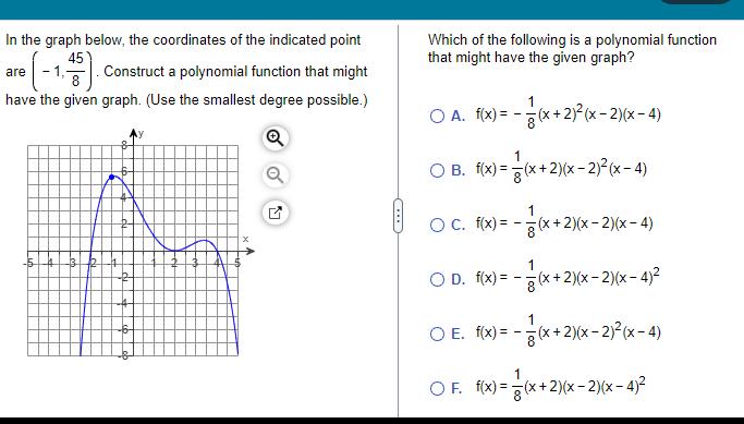
Quadratic equationsIn the graph below the coordinates of the indicated point are 1 1 45 Construct a polynomial function that might have the given graph Use the smallest degree possible Q 13 R Ly Which of the following is a polynomial function that might have the given graph O A f x x 2 x 2 x 4 1 O B f x x 2 x 2 x 4 1 OC f x x 2 x 2 x 4 O D f x O E f x x 2 x 2 x 4 1 x 2 x x 2 x 2 x 4 OF f x x 2 x 2 x 4
Algebra
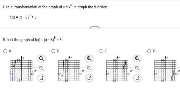
Quadratic equationsUse a transformation of the graph of y x5 to graph the function f x x 8 5 5 Select the graph of f x x 8 5 5 O A Q O B Q O C

Algebra
Matrices & DeterminantsvausvAI The objective function is maximization so the resulting LPP becomes Max z 5x 3x 0x3 0x4 0x5 subject to X x2 x3 2 5x 2x x 10 3x1 8x2 x5 12 x 20 Vi 1 2 5 The initial basic feasible solution is obtained by putting x x2 0 in the reformulated form of LPP and we get x3 2 x4 10 x5 12 Starting Simplex Table 000 CB XB 5 0 0 1 X3 2 Y3 X4 10 Y4 5 X5 12 Y5 2 First Iteration CB 72 CBi Yij B1 Z G Z C YB XB X 2 X4 0 X5 6 New Pivot equation old equation pivot element Z 0 72 CBi Xij j 1 2 9 5 C YB Y 1 Y 0 Ys 0 5 5 0 Y 5 Y 1 2 8 0 3 1 3 5 5 2 7 3 Y 3 Y 1 0 0 0 0 1 5 3 5 5 0 Y3 0 Y3 Hence an optimal basic feasible solution is obtained Solution is x 2 x 0 and Max z 10 Exercise 0 1 0 0 0 0 1 0 0 0 0 Y 0 Y 0 0 1 0 0 0 0 1 0 0 1 Solve the following LPP using simplex method Min z x 3x2 2x3 subject to 3x1 x2 2x3 7 0 Y 0 Y Ratio 2 2 4 XBi Yir 2x 4x2 12 4x 3x2 8x3 10 and x 0 Vi 1 2 3 2 Solve the following LPP using simplex method

Algebra
Matrices & DeterminantsThe objective function is converted to maximisation objective function The resulting LPP becomes Max z 12x 20x 0x3 0x4 Mx5 Mx subject to 6x1 8x2x3 x5 100 7x1 12x2x4 x6 120 xi 20 Vi The initial basic feasible solution is obtained by putting x x x3 X4 0 in the reformulated form of LPP and we get x5 100 x6 120 Starting Simplex Table CB M M M 20 XB X5 100 Y X6 120 Y6 n First Iteration Z CBiYij j 1 Z G 12 20 CB XB X5 20 Y5 X 10 Y Second Iteration C YB Y CB XB X 15 X 5 4 n z CBt Yij Z Gj 72 12 6 7 13M G 12 YB Y 13M 20 4 3 7 12 4M 3 1 3 C YB Y 1 Y 0 z CBiY ij 7 1 4 G 12 Y 12 0 4M 3 35 3 20 0 1 20 8 12 20M 9 Y 20M 20 0 20 Y 0 20 Y 0 1 20 0 Y3 1 0 M M ol 0 Y3 1 0 M M 0 Y3 3 4 7 16 14 14 0 Y 0 1 M M 10 0 Y4 2 3 1 12 2M 5 5 3 2M 5 5 3 1 0 M 0 Y4 7 3 0 5 12 7 3 Hence an optimal basic feasible solution is obtained Solution is x 15 x 5 4 and Max z 205 M M Ratio Y5 Y5 1 0 M Y6 0 1 M 0 M Ratio 0 XBi Yir 12 5 10 XBi Yir 15 120 7

Algebra
Matrices & DeterminantsThe initial basic feasible solution is obtained by putting x x x3 X4 0 in the reformulated form of LPP and we get x5 900 x6 1200 Starting Simplex Table CB M M CB First Iteration M 60 CB 80 60 XB X5 900 Ys 20 X6 1200 Y 40 60M z CBi Yij j 1 Z Gj XB X 300 X 30 Second Iteration C 5 72 C YB 72 z CBi Yij 1 Z G Y Y6 Y C YB z CBiYij 1 Z G 60 Y 60M 60 0 0 1 60 60 Y XB X 20 Y 0 X 15 Y 1 60 Y 60 0 11 30 30 60M 80 60M 80 15 3 4 Y 80 Y 15M 45 0 15M 35 80 Y 1 0 80 12 0 Y3 Y 1 0 M 0 M M 1 0 M M 0 0 Y3 1 15 1 20 7 3 0 1 M Y3 Y4 7 3 HHH 0 lo M 2 3 2 M 2 3 2 1 3 Hence an optimal basic feasible solution is obtained Solution is x 15 x 20 and Max 2 2500 M M Ys 1 0 1 M M 0 Y4 1 30 1 20 1 3 0 1 2 1 1 40 0 0 M Y5 M Y 0 0 Ratio Ratio XBi Yir 20 40 45 30 XBi Yir

Algebra
Matrices & Determinantsvausva The objective function is maximization so the resulting LPP becomes Max z 5x 3x 0x3 0x4 0x subject to x x2 x3 2 5x 2x x 10 3x1 8x2 x5 12 x 0 Vi 1 2 5 The initial basic feasible solution is obtained by putting x x2 0 in the reformulated form of LPP and we get x3 2 x4 10 x5 12 Starting Simplex Table 000 CB XB 5 0 0 1 X3 2 Y3 X4 10 Y4 5 X5 12 Y5 2 First Iteration CB 72 CBi Yij B1 Z G Z C YB XB X 2 X4 0 X5 6 New Pivot equation old equation pivot element Z 0 72 CBi Xij j 1 2 9 5 C YB Y 1 Y 0 Ys 0 5 5 0 Y 5 Y 1 2 8 0 3 1 3 5 5 2 7 3 Y 3 Y 1 0 0 0 0 1 5 3 5 5 0 Y3 0 Y3 Hence an optimal basic feasible solution is obtained Solution is x 2 x 0 and Max z 10 Exercise 0 1 0 0 0 0 1 0 0 0 0 Y 0 Y 0 0 1 0 0 0 0 1 0 0 1 Solve the following LPP using simplex method Min z x 3x2 2x3 subject to 3x1 x2 2x3 7 0 Y 0 Y Ratio 2 2 4 XBi Yir 2x 4x2 12 4x 3x2 8x3 10 and x 0 Vi 1 2 3 2 Solve the following LPP using simplex method

Algebra
Complex numbers3 20 3 18 10 Step 6 Sixth allocate in 3 4 cell X34 min 5 5 5 4 18 5 5 3 The initialz basic feasible solution is given by X11 5 X12 10 X22 5 X23 15 X24 5 X34 5 1 2 3 4 5 10 1 5 2 3 b 1 2 3 1 6 8 9 4 6 10 12 14 16 18 Minimum transportation cost 5 10 10 0 5 7 15 9 5 20 5 18 Rs 410 Exercise 1 Using North West Corner rule find out the initial basic feasible solution to the following TP 2 Least Cost Method 5 0 0 2 3 4 a 4 1 5 14 15 2 7 16 3 6 2 5 10 15 4 35 20 7 9 20 5 20 11 5 The procedure is as follows Step 1 Determine the smallest cost in the cost matrix of the transportation table Let it be Cij Allocate x min a b in the i j cell Step 2 If x j a cross off ith row of the transportation table and decrease b by aj If xij b cross off jth column of the transportation table and decrease a by bj If Xij a bj cross off either the first row or the first column but not both Step 4 Reneat stens 1 and 2 for the resulting table Reduce transportation table
Algebra
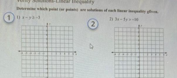
Quadratic equationsInequality Determine which point or points are solutions of each linear inequality given 1 1 x y2 3 2 3x 5y 10 2 27 0436 AT

Algebra
Permutations and CombinationsThe procedure is as follows Step 1 Start with the cell 1 1 at the north west corner of the transportation table and allocate it maximum possible amount x 1 min a b so that either the capacity of the origin O or the requirement for the destination D satisfies it or both Step 2 If X a cross off the first row of the transportation table and decrease b by a and go to step 3 If X 1 b cross off the first column of the transportation table and decrease a by by and go to step 3 If x a b cross off either the first row or the first column but not both Step 3 Repeat steps 1 and 2 for the resulting reduced transportation table until all the requirements are satisfied Note The N W corner rule of allocating values of the variables eliminates either a row or column of the table from further consideration and the last allocation eliminates both a row and column Hence a feasible solution obtained by this method has m n 1 basic variables Problem Find an initial basic feasible solution to the following TP using North West Comer Rule Solution 1 2 3 b a 1 2 3 F 1 10 0 2 Step 1 First allocate in 1 1 cell X 1 min 15 5 5 12 7 3 2 1 3 4 a 15 20 11 0 14 16 18 5 5 15 15 10 45 9 20 25 b 5 2 3 4 10 0 20 11 15 18 12 7 9 20 25 Step 2 Second allocate in 1 2 cell X 2 min 10 15 10 2 3 4 0 2011 10 0 14 16 18 5 15 15 1 45 7 9 20 25 14 16 18 5 5 15 10 Step 3 Third allocate in 2 2 cell X min 25 5 5
Algebra
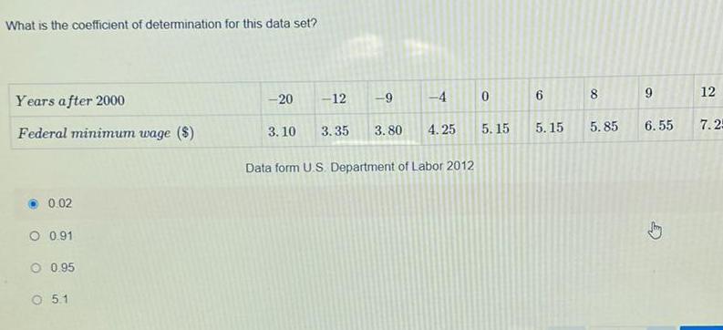
Sequences & SeriesWhat is the coefficient of determination for this data set Years after 2000 Federal minimum wage 0 02 O 0 91 0 95 O 5 1 20 3 10 12 3 35 4 3 80 4 25 9 Data form U S Department of Labor 2012 0 5 15 6 5 15 00 8 5 85 9 6 55 Jhy 12 7 25

Algebra
Quadratic equationsWhich phrase identifies the importance of the elastic clause in Article 1 Provides a loophole to make laws without the approval of the executive branch O Gives Congress powers that stretch beyond the other branches of government ORemoves flexibility to legislate on topics not listed in the Constitution O Allows Congress to make laws not specifically stated in the Constitution

Algebra
Permutations and CombinationsThe minimum processing time among these jobs is 6 which corresponds to the job J4 on machine M and job J5 on machine M Hence J4 is placed in the first available position in the sequence as shown below J2 J4 J5 Finally the job J3 is placed as shown below J2 J4 J3 Thus J2J4J3 two machines Sequencing n Jobs on 3 Machines Processing n Jobs in m Machines Machines M M M3 J5 J J5J is the optimal sequence of the five jobs on the Let there be n jobs J IzIn each of which is to be processed in m machines say M M Mm in the order M M Mm The list of job numbers 1 2 n with their processing time is given in the following table Job numbers 1 t11 t21 t31 3 t13 t22 t23 t32 33 2 t12 J En tin tzn t3n Mm tmn tm1 tm3 An optimum solution to this problem can be obtained if either or both of the following conditions are satisfied a min t max ty for i 2 3 k 1 b min tj 2 max ty for i 2 3 k 1 35 If the above condition is satisfied then the problem can be converted to an equivalent two machines and n jobs problem Algorithm for optimum sequence for n jobs in m machines The iterative procedure for determining the optimal sequence for n jobs in m machines is given below Step 1 Find min tij and mintmj Also find the maximum of each of t2j t3j t for all j 1 2 n Step 2 Check the following a min ti 2 max tij for i 2 3 k 1 b min tm max tij for i 2 3 k 1 Step 3 If both the inequalities of step 2 are not satisfied this method fails
Algebra
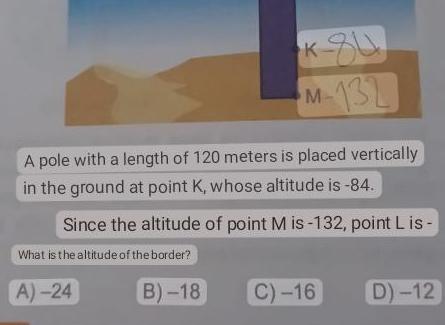
Quadratic equationsA pole with a length of 120 meters is placed vertically in the ground at point K whose altitude is 84 Since the altitude of point M is 132 point Lis What is the altitude of the border K 84 M 132 A 24 B 18 C 16 D 12

Algebra
Complex numbersNow we find the optimum sequence of the 6 jobs in two machines H and Kas usual in the following tables J4 J4 J4 J4 3 3 J3 Job seq J J J6 J 16 J3 J J6 J2 Js Jz Hence the optimal sequencing is J 13 1 16 12 15 Table to find minimum elapsed time Js Total M Time in Time out J5 Js out 0 2 2 8 7 10 12 10 21 21 21 33 33 33 42 42 17 8 2 7 M Time in Time 37 45 M3 Idle Idle time time M M3 Time in Time out 8 8 20 2 12 20 29 20 29 42 22 42 55 1 39 55 69 11 69 77 3 Minimum total elapsed time 77 Hrs Idle time for M 77 42 35 Idle time for M 17 77 45 17 32 49 8 0 0 0 0 0

Algebra
Matrices & Determinants7 Which of the following phenomena of light are involved in the formation of a rainbow A Refraction B Dispersion C Internal reflection Only one correct answer A A and B only B B and C only C D A and C only Review All A B and C 0
Algebra
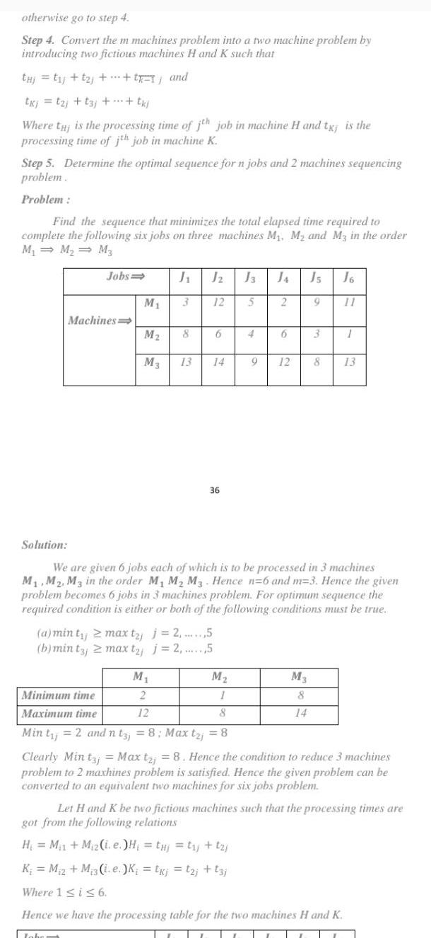
Sequences & Seriesotherwise go to step 4 Step 4 Convert the m machines problem into a two machine problem by introducing two fictious machines H and K such that thi t j t j tk and U tkj 12 t3j tkj Where tj is the processing time of jth job in machine H and tx is the processing time of jth job in machine K Step 5 Determine the optimal sequence for n jobs and 2 machines sequencing problem Problem Find the sequence that minimizes the total elapsed time required to complete the following six jobs on three machines M M and M3 in the order M M M3 Jobs Machines J Jz M 3 12 M 8 M3 13 6 a min ty 2 max t j j 2 5 b min tj 2 max t j j 2 5 M 2 12 14 36 J3 5 M 1 8 4 2 6 Js J6 11 9 3 9 12 8 Solution We are given 6 jobs each of which is to be processed in 3 machines M M2 M3 in the order M M M3 Hence n 6 and m 3 Hence the given problem becomes 6 jobs in 3 machines problem For optimum sequence the required condition is either or both of the following conditions must be true M3 8 14 1 13 Minimum time Maximum time Min t 2 and nt3j 8 Max taj 8 Clearly Min t3 Max t 8 Hence the condition to reduce 3 machines problem to 2 maxhines problem is satisfied Hence the given problem can be converted to an equivalent two machines for six jobs problem Hence we have the processing table for the two machines H and K Jober Let H and K be two fictious machines such that the processing times are got from the following relations H M M z i e H tj tj t j K M 2 M 3 i e K txj tzi t3j Where 1 i 6
Algebra
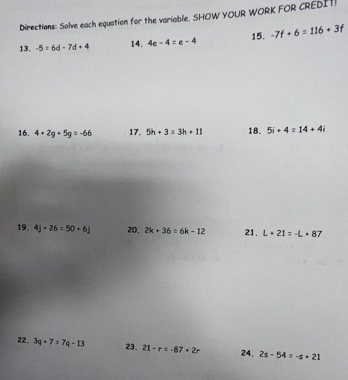
Quadratic equationsDirections Solve each equation for the variable SHOW YOUR WORK FOR CRED 13 56d 7d 4 15 7f 6 116 3f 16 4 2g 5g 66 19 4j 26 50 6j 22 3q 7 7q 13 14 4e 4 e 4 17 5h 3 3h 11 20 2k 36 6k 12 23 21 r 87 2r 18 5i 4 14 4i 21 L 21 L 87 24 2s 54 s 21
Algebra
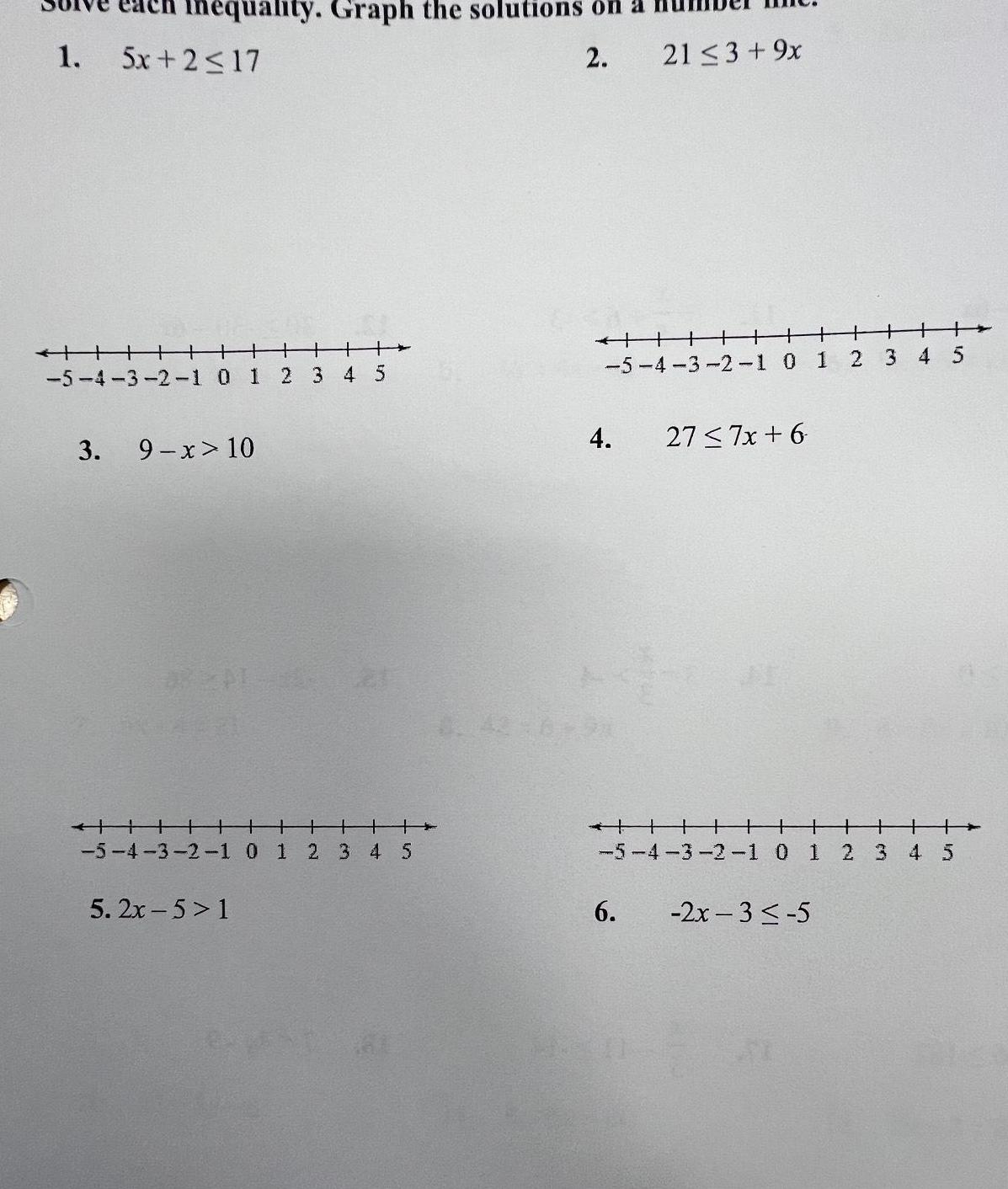
Quadratic equations1 nequality Graph the solutions on 2 5x 2 17 TH1 5 4 3 2 1 0 1 2 3 4 5 3 9 x 10 5 4 3 2 1 0 1 2 3 4 5 5 2x 5 1 HHHHH 21 3 9x 5 4 3 2 1 0 1 2 3 4 5 4 6 27 7x 6 5 4 3 2 1 0 1 2x 3 5 2 3 4 5
Algebra
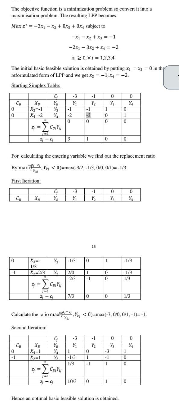
Quadratic equationsThe objective function is a minimization problem so convert it into a maximisation problem The resulting LPP becomes Max z 3x x2 0x3 0x4 subject to X1X2 x3 1 2x13x2 x4 2 Xi 0 Vi 1 2 3 4 The initial basic feasible solution is obtained by putting x x2 0 in the reformulated form of LPP and we get x3 1 x4 2 Starting Simplex Table 0 0 0 CB 1 XB X 1 X4 2 First Iteration CB 0 1 Zj Z CB 71 n 7731 Z C XB X3 1 3 X 2 3 Second Iteration C YB Y Y Y3 Y Z CBi Yij j 1 2 G 72 XB X 1 X 1 CBi Yij For calculating the entering variable we find out the replacement ratio By max kj 0 max 3 2 1 3 0 0 0 1 1 3 72 C 1 2 0 3 3 Y Z CBiYij j 1 Z cj 3 Y 1 3 2 0 2 3 7 3 C YB Y 1 Y 1 3 1 3 3 Y 1 3 0 1 10 3 0 1 1 0 1 Y 0 1 1 0 1 Y 15 1 0 0 0 1 Y 1 7 9 Calculate the ratio max kj 0 max 7 0 0 0 1 1 1 Ykj 0 0 0 0 Y3 3 1 1 1 0 Y 0 1 0 0 Y3 0 Hence an optimal basic feasible solution is obtained 0 Y 1 3 0 Y 1 3 1 3 1 3 1 0 0 0 0 Y
Algebra
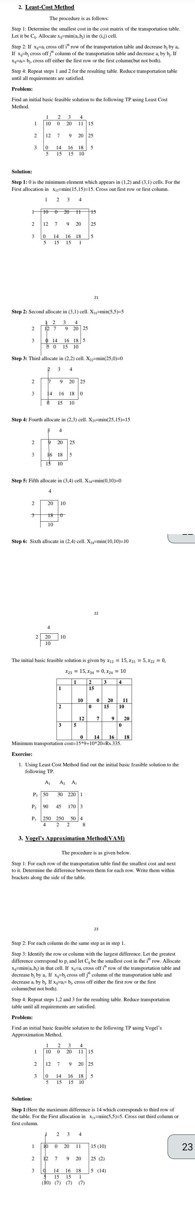
Sequences & Series2 Least Cost Method The procedure is as follows Step 1 Determine the smallest cost in the cost matrix of the transportation table Let it be Cij Allocate x j min a b in the ij cell Step 2 If x j a cross off ith row of the transportation table and decrease b by a If x b cross off jh column of the transportation table and decrease a by bj If Xij a bj cross off either the first row or the first column but not both Step 4 Repeat steps 1 and 2 for the resulting table Reduce transportation table until all requirements are satisfied Problem Find an initial basic feasible solution to the following TP using Least Cost Method 1 2 3 F 2 Solution Step 1 0 is the minimum element which appears in 1 2 and 3 1 cells For the First allocation in X 2 min 15 15 15 Cross out first row or first column 1 3 4 3 2 3 2 3 2 3 I 2 3 4 10 0 20 11 15 2 12 7 9 20 25 Step 2 Second allocate in 3 1 cell X 1 min 5 5 5 12 3 4 12 7 3 0 14 16 18 5 5 15 15 10 10 0 20 H 12 7 9 20 0 5 15 15 1 Step 3 Third allocate in 2 2 cell X 2 min 25 0 0 2 3 4 2 Solution 14 16 18 5 14 5 0 15 10 Step 4 Fourth allocate in 2 3 cell X23 min 25 15 15 7 9 20 25 14 16 18 0 0 15 10 B 4 3 Step 5 Fifth allocate in 3 4 cell X34 min 0 10 0 4 1 9 20 25 16 18 5 15 10 4 2 20 10 18 10 9 20 25 16 18 5 20 10 Step 6 Sixth allocate in 2 4 cell X24 min 10 10 10 0 The initial basic feasible solution is given by x12 15 X31 5 x22 0 X23 15 X34 0 X24 10 1 3 4 10 1 2 d 3 A A P 50 30 220 1 P 90 45 170 3 P 250 250 50 4 4 2 2 8 1 2 1 10 0 10 5 10 15 12 25 0 14 16 18 Minimum transportation cost 15 9 10 20 Rs 335 Exercise 1 Using Least Cost Method find out the initial basic feasible solution to the following TP 0 3 Vogel s Approximation Method VAM 20 The procedure is as given below Step 1 For each row of the transportation table find the smallest cost and next to it Determine the difference between them for each row Write them within brackets along the side of the table 21 Step 2 For each column do the same step as in step 1 Step 3 Identify the row or column with the largest difference Let the greatest difference correspond to p and let Cij be the smallest cost in the ith row Allocate x min a b in that cell If xa cross off ith row of the transportation table and decrease b by a If x b cross off jth column of the transportation table and decrease a by bj If xa b cross off either the first row or the first column but not both 3 4 2 3 Step 4 Repeat steps 1 2 and 3 for the resulting table Reduce transportation table until all requirements are satisfied 0 Problem Find an initial basic feasible solution to the following TP using Vogel s Approximation Method 2 12 7 9 20 25 2 15 22 0 14 16 18 5 5 15 15 10 11 15 4 0 20 11 15 10 7 20 11 Step 1 Here the maximum difference is 14 which corresponds to third row of the table For the First allocation in X min 5 5 5 Cross out third column or first column 9 20 0 23 15 10 2 12 7 9 20 25 2 3 a 14 16 18 5 14 15 15 1 10 7 7 7 23

Algebra
Complex numberst Light is Ligh articles 1 particte photon has energy Quantum TQuantum I photon a form of as energy Radiation energy Asafasa Electric field magnetic field light partides also light is particle wave behave as when light proticle move they mo duce Electric magnetic field he which as perpendicular Do light are considere an electromagnetic wave Speed 3 0 x108 m see Energy of Single photon 1 Energy ho s cycter wave per do Second planck s constant 6 626 110 7

Algebra
Matrices & Determinantsis a px p symmetric matrix with spectral decomposition A FAIT where diag A show that det A tr A

Algebra
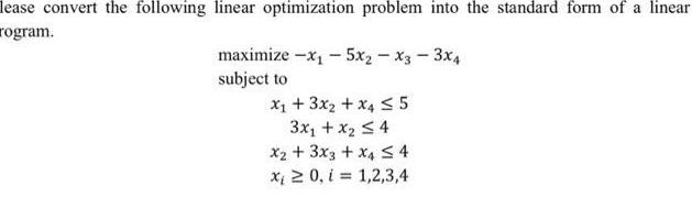
Sequences & Serieslease convert the following linear optimization problem into the standard form of a linear rogram maximize x 5x x3 3x4 subject to x 3x x4 5 3x x 4 x 3x3 x4 4 x 0 i 1 2 3 4

Algebra
Complex numbersAt the age of 24 to save for retirement you decide to deposit 10 at the end of each month in an IRA that pays 5 5 compounded monthly a b Use the following formula to determine how much you will have in the IRA when you retire at age 65 P 1 r 1 A A P nt A Find the interest or a You will have approximately in the IRA when you retire Do not round until the final answer Then round to the nearest dollar as needec

Algebra
Permutations and Combinationsale formula to find the value of the annuity Find the interest Periodic Deposit 70 at the end of each month Rate 7 compounded monthly Click the icon to view some finance formulas a The value of the annuity is Do not round until the final answer Then round to the nearest dollar as needed Formulas A Time 30 years In the provided formulas P is the deposit made at the end of each compounding period r is the annual interest rate of the annuity in decimal form n is the number of compounding periods per year and A is the value of the annuity after t years P 1 r 1 nt P 1 2 1 n A P A 9 nt 1
Algebra
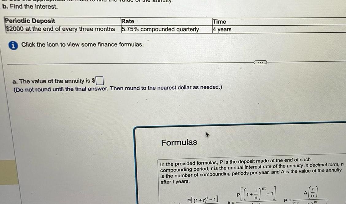
Sequences & Seriesb Find the interest Periodic Deposit Rate 2000 at the end of every three months 5 75 compounded quarterly Click the icon to view some finance formulas Time 4 years a The value of the annuity is Do not round until the final answer Then round to the nearest dollar as needed Formulas In the provided formulas P is the deposit made at the end of each compounding period r is the annual interest rate of the annuity in decimal form n is the number of compounding periods per year and A is the value of the annuity after t years P 1 r 1 nt 1 P P A n nt