Algebra Questions
The best high school and college tutors are just a click away, 24×7! Pick a subject, ask a question, and get a detailed, handwritten solution personalized for you in minutes. We cover Math, Physics, Chemistry & Biology.
Algebra
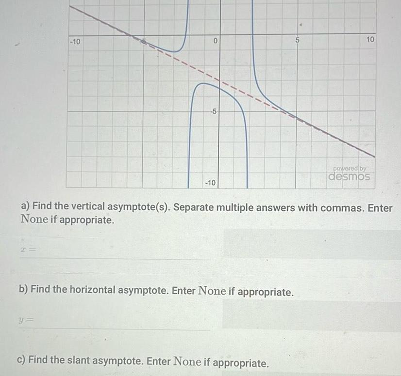
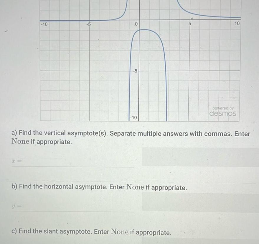
Quadratic equations2 10 O y 5 10 b Find the horizontal asymptote Enter None if appropriate a Find the vertical asymptote s Separate multiple answers with commas Enter None if appropriate 10 c Find the slant asymptote Enter None if appropriate 10 powered by desmos
Algebra
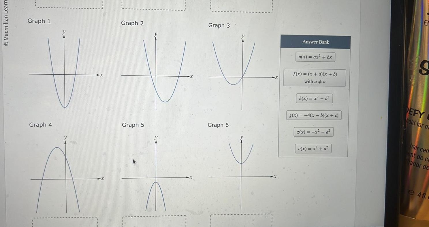
Quadratic equationsO Macmillan Learn Graph 1 Graph 4 Graph 2 Graph 5 Graph 3 Graph 6 Answer Bank u x ax bx f x x a x b with a b h x x b g x 4 x b x c z x x a v x x a m B S DEFY hold for m hair cem ent de ch ador de e 4fl c
Algebra
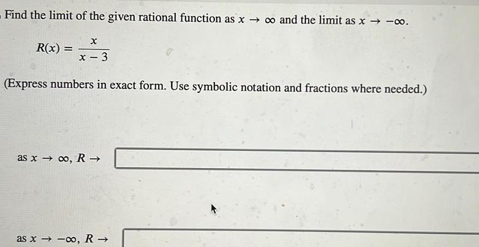
Quadratic equationsFind the limit of the given rational function as x o and the limit as x co R x X x 3 Express numbers in exact form Use symbolic notation and fractions where needed as x o R as x o R
Algebra
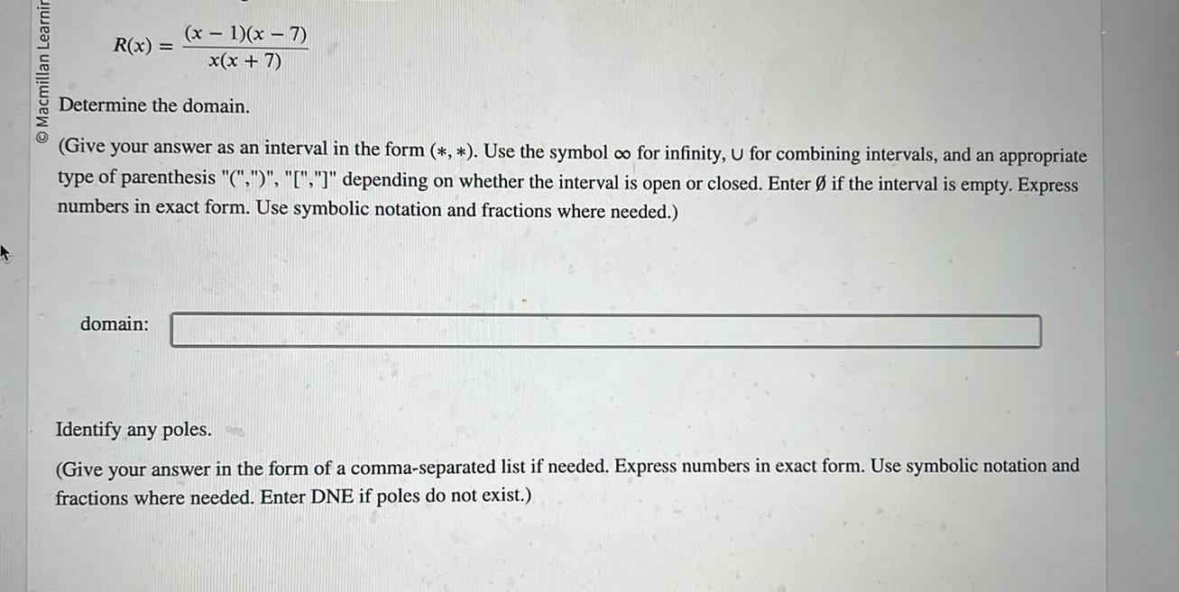
Quadratic equationsO Macmillan Learnir x 1 x 7 R x x x 7 Determine the domain Give your answer as an interval in the form Use the symbol co for infinity U for combining intervals and an appropriate type of parenthesis depending on whether the interval is open or closed Enter if the interval is empty Express numbers in exact form Use symbolic notation and fractions where needed domain Identify any poles Give your answer in the form of a comma separated list if needed Express numbers in exact form Use symbolic notation and fractions where needed Enter DNE if poles do not exist
Algebra
Quadratic equations10 5 y 0 5 10 b Find the horizontal asymptote Enter None if appropriate 5 a Find the vertical asymptote s Separate multiple answers with commas Enter None if appropriate c Find the slant asymptote Enter None if appropriate 10 powered by desmos
Algebra
Quadratic equationsUse a calculator to evaluate the expression to the nearest tenth of a degree sin 0 1302
Algebra
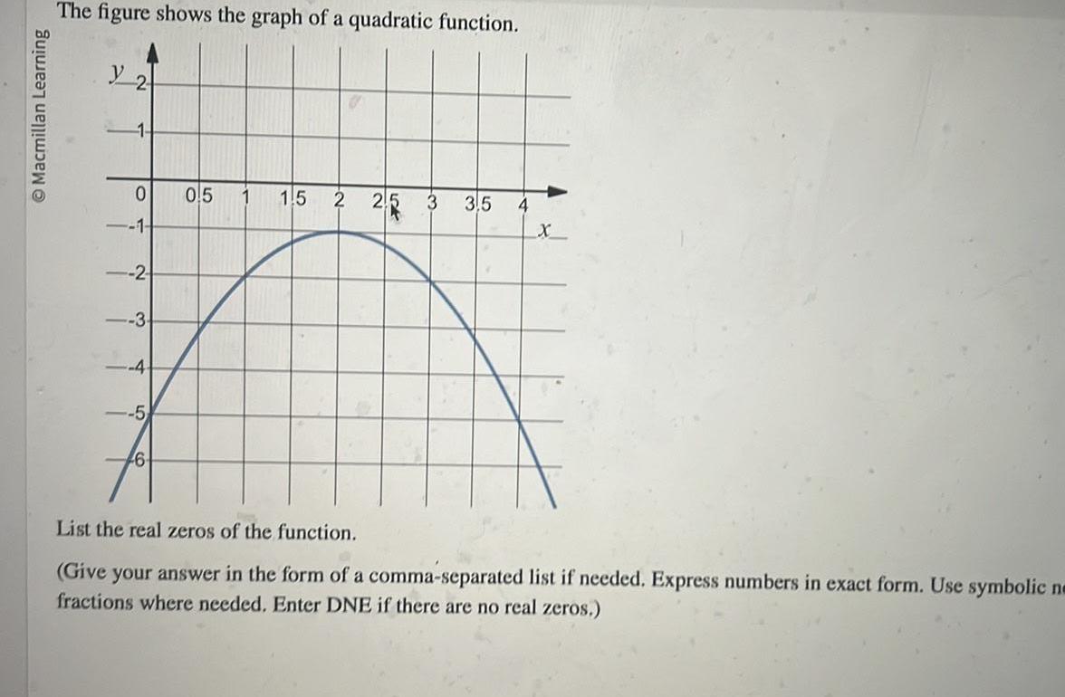
Quadratic equationsMacmillan Learning The figure shows the graph of a quadratic function y 2 1 0 1 2 3 4 5 6 0 5 1 5 2 25 3 3 5 4 X List the real zeros of the function Give your answer in the form of a comma separated list if needed Express numbers in exact form Use symbolic ne fractions where needed Enter DNE if there are no real zeros
Algebra
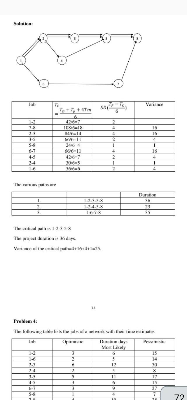
Quadratic equationsSolution Job 1 2 7 8 2 3 3 5 5 8 6 7 4 5 2 4 1 6 6 1 2 3 TE The various paths are 1 2 1 6 2 3 2 4 3 5 4 5 6 7 5 8 78 TD Tp 4Tm 6 42 6 7 108 6 18 84 6 14 66 6 11 24 6 4 66 6 11 42 6 7 30 6 5 36 6 6 The critical path is 1 2 3 5 8 The project duration is 36 days Variance of the critical path 4 16 4 1 25 3 2 1 2 3 5 8 1 2 4 5 8 1 6 7 8 6 2 5 3 3 1 A 73 5 SD Tp 6 2 4 4 2 1 4 2 1 2 6 7 Problem 4 The following table lists the jobs of a network with their time estimates Job Optimistic Duration days Most Likely 5 12 5 11 6 9 4 10 Variance 16 16 4 1 16 4 1 4 Duration 36 23 35 Pessimistic 15 14 30 8 17 15 27 7 25 72
Algebra
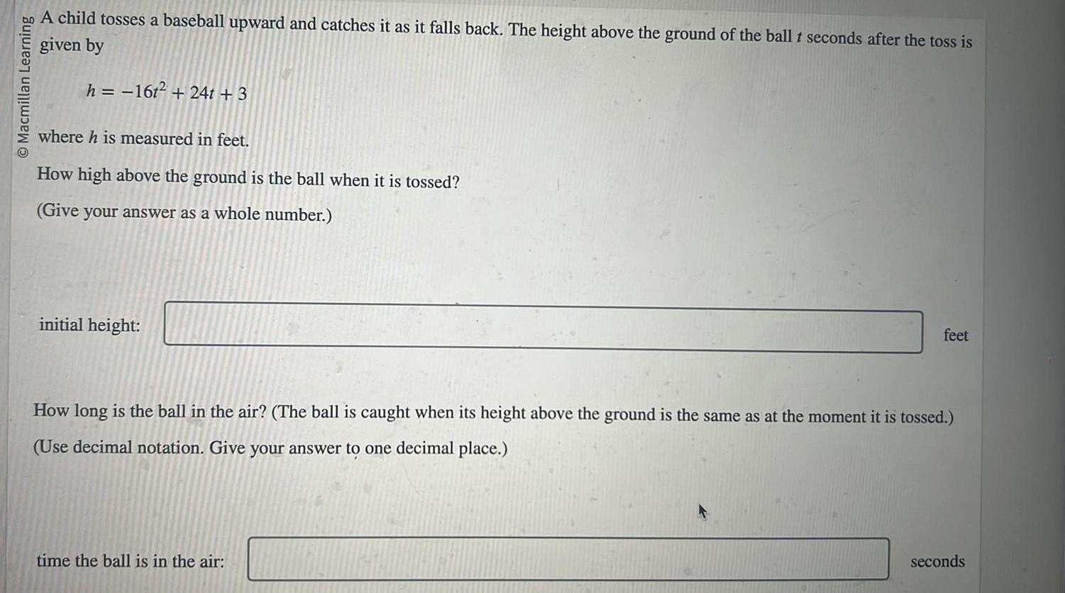
Quadratic equationsO Macmillan Learning A child tosses a baseball upward and catches it as it falls back The height above the ground of the ball t seconds after the toss is given by h 16t 24t 3 where h is measured in feet How high above the ground is the ball when it is tossed Give your answer as a whole number initial height feet How long is the ball in the air The ball is caught when its height above the ground is the same as at the moment it is tossed Use decimal notation Give your answer to one decimal place time the ball is in the air seconds
Algebra
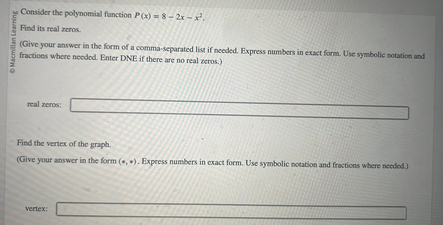
Quadratic equationsMacmillan Learning Consider the polynomial function P x 8 2x x Find its real zeros Give your answer in the form of a comma separated list if needed Express numbers in exact form Use symbolic notation and fractions where needed Enter DNE if there are no real zeros real zeros Find the vertex of the graph Give your answer in the form Express numbers in exact form Use symbolic notation and fractions where needed vertex
Algebra
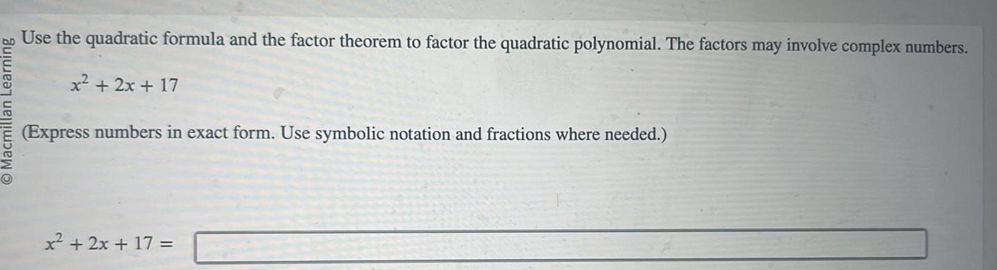
Complex numbersO Macmillan Learning Use the quadratic formula and the factor theorem to factor the quadratic polynomial The factors may involve complex numbers x 2x 17 Express numbers in exact form Use symbolic notation and fractions where needed x 2x 17
Algebra
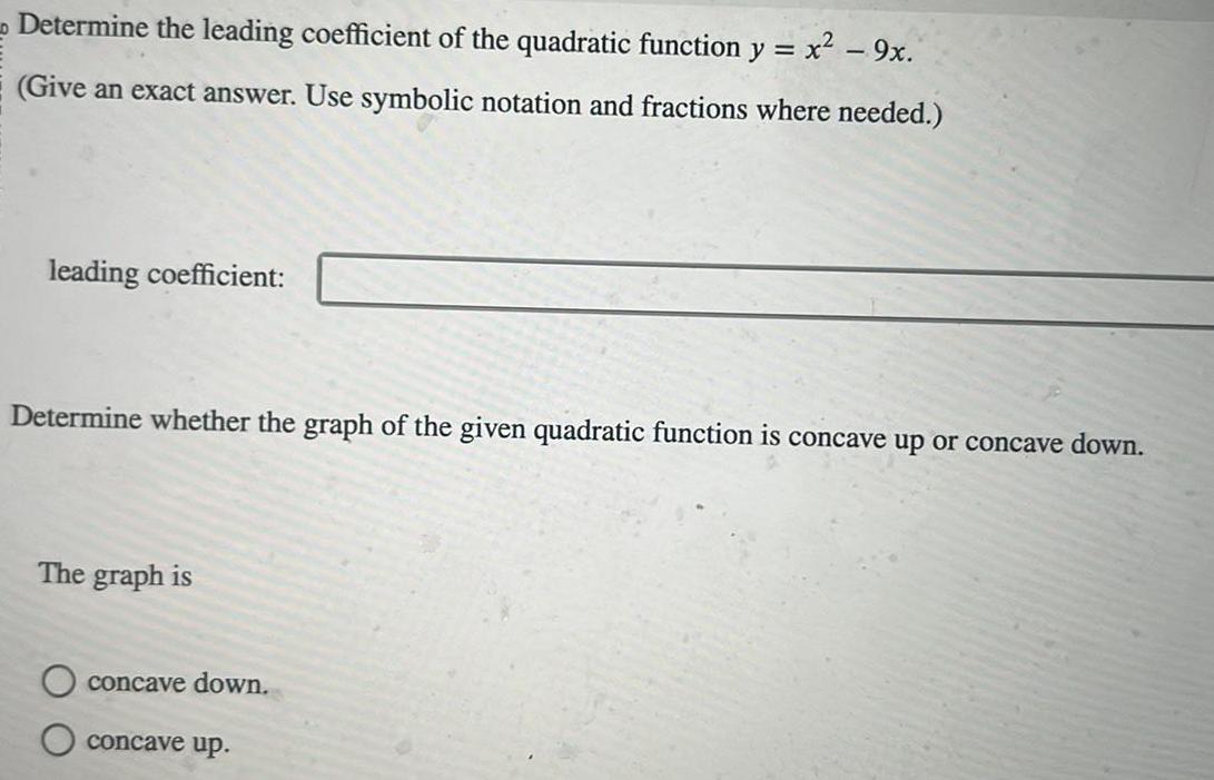
Complex numbersDetermine the leading coefficient of the quadratic function y Give an exact answer Use symbolic notation and fractions where needed leading coefficient Determine whether the graph of the given quadratic function is concave up or concave down The graph is concave down x 9x concave up
Algebra
Quadratic equationsMacmillan Learning Calculate the discriminant of the quadratic function y x 3x 4 Give an exact answer Use symbolic notation and fractions where needed discriminant What does the discriminant tell you about the zeros The equation has one real zero Otwo real zeros no real zeros
Algebra
Quadratic equationsMultiply the factors and simplify the expression x 6 i x 6 i Suggestion Use the fact that A B A B A B Express numbers in exact form Use symbolic notation and fractions where needed Simplify your answer completely x 6 i x 6 i
Algebra
Complex numbersMacmillan Learning Find the vertex of the parabola y x 4x 10 Give your answer in the form Express numbers in exact form Use symbolic notation and fractions where needed vertex Indicate whether the vertex corresponds to a maximum or a minimum minimum maximum

Algebra
Sequences & Seriesii 6 pt Find the inverse function of f x 3sinx 1 where sxs then find the range of f and the range and domain off
Algebra
Complex numbersMacmillan Learning Write the polynomial P x with zeros x 2 and x 6 and with leading coefficient 3 in factored form Express numbers in exact form Use symbolic notation and fractions where needed P x
Algebra
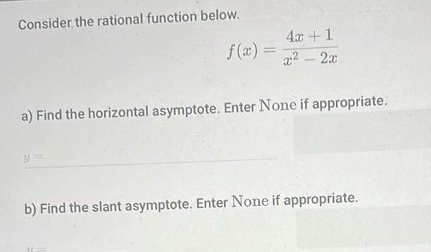
Quadratic equationsConsider the rational function below f x 4x 1 x 2x a Find the horizontal asymptote Enter None if appropriate b Find the slant asymptote Enter None if appropriate
Algebra
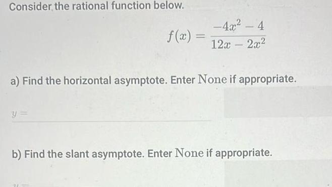
Complex numbersConsider the rational function below 4x 4 12x 2x a Find the horizontal asymptote Enter None if appropriate y b Find the slant asymptote Enter None if appropriate
Algebra
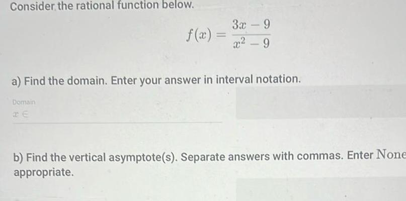
Complex numbersConsider the rational function below f x Domain 3x 9 x 9 a Find the domain Enter your answer in interval notation b Find the vertical asymptote s Separate answers with commas Enter None appropriate
Algebra
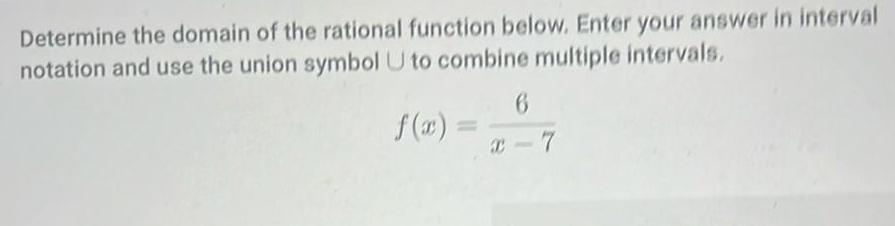
Quadratic equationsDetermine the domain of the rational function below Enter your answer in interval notation and use the union symbol U to combine multiple intervals f x C 6
Algebra
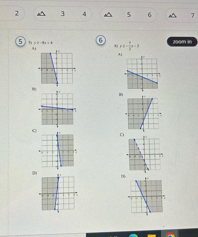
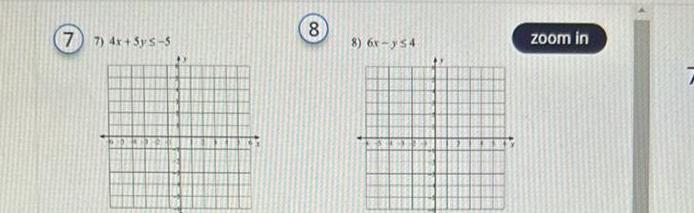
Quadratic equations1 2 3 here to search 3 9x 4y5 16 A B 5 A D 3 4 C 4 A 5 6 4 2 3x 3 A A zoom in 7 8
Algebra
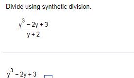
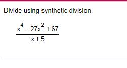
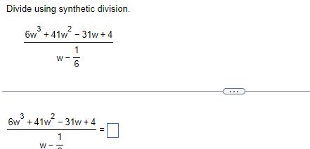
Quadratic equationsDivide using synthetic division 3 2 6w 41w 31w 4 W W 1 6 6w 41w 2 31w 4 3 1
Algebra
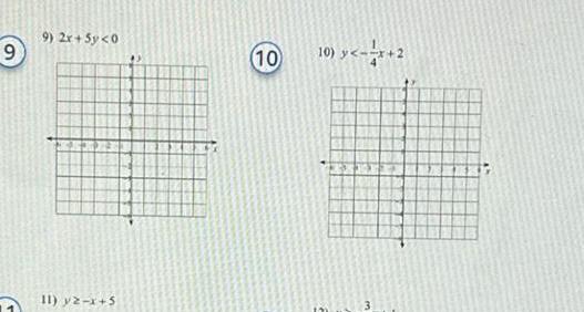
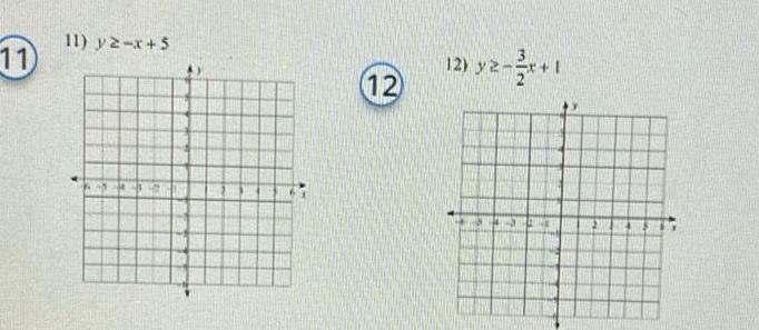
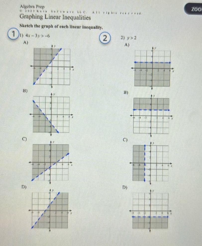
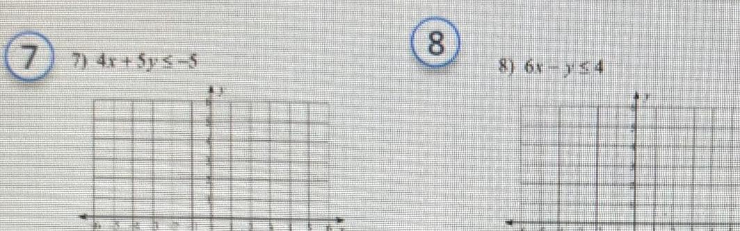
Complex numbers1 Algebra Prep 2023 Kia Software LLC ATT right re Graphing Linear Inequalities Sketch the graph of each linear inequality 4x 3y 6 A B D 2 2 y 2 A B C D D X ZOOL
Algebra
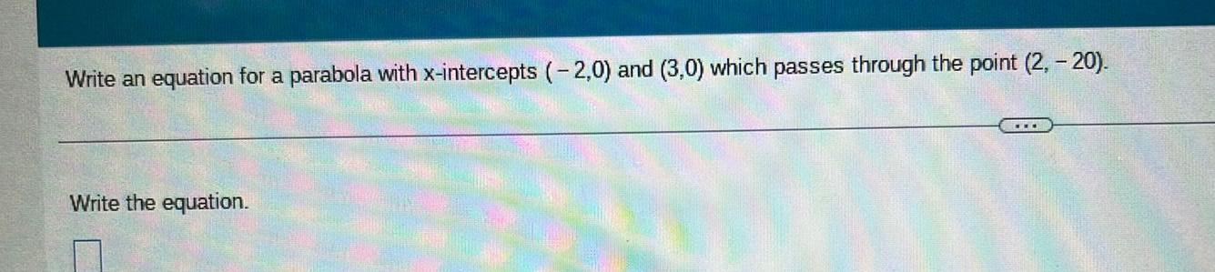
Quadratic equationsWrite an equation for a parabola with x intercepts 2 0 and 3 0 which passes through the point 2 20 Write the equation
Algebra
Complex numbersMultiply 2i 4 5i 2i 4 5i Simplify your answer Type your answer in the form a bi
Algebra
Permutations and CombinationsMultiply 3i 3i 3i 3i 0 Simplify your answer Type your answer in the form a bi
Algebra
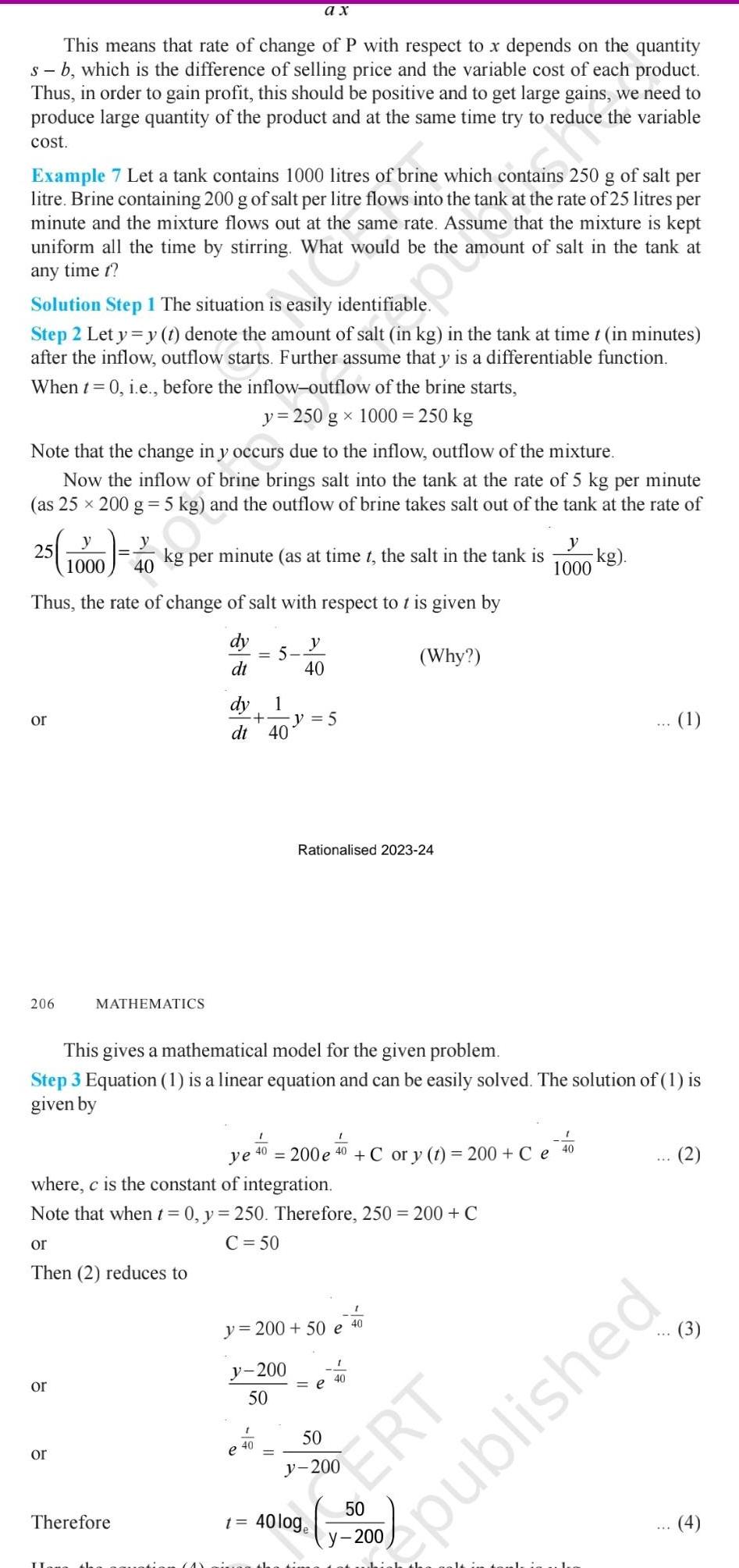
Matrices & DeterminantsThis means that rate of change of P with respect to x depends on the quantity s b which is the difference of selling price and the variable cost of each product Thus in order to gain profit this should be positive and to get large gains we need to produce large quantity of the product and at the same time try to reduce the variable cost Example 7 Let a tank contains 1000 litres of brine which contains 250 g of salt per litre Brine containing 200 g of salt per litre flows into the tank at the rate of 25 litres per minute and the mixture flows out at the same rate Assume that the mixture is kept uniform all the time by stirring What would be the amount of salt in the tank at any time t Solution Step 1 The situation is easily identifiable Step 2 Let y y t denote the amount of salt in kg in the tank at time t in minutes after the inflow outflow starts Further assume that y is a differentiable function When t 0 i e before the inflow outflow of the brine starts y 250 g x 1000 250 kg Note that the change in y occurs due to the inflow outflow of the mixture Now the inflow of brine brings salt into the tank at the rate of 5 kg per minute as 25 x 200 g 5 kg and the outflow of brine takes salt out of the tank at the rate of 25 or 206 00 4 1000 Thus the rate of change of salt with respect to t is given by dy Why dt or or 40 kg per minute as at time t the salt in the tank is MATHEMATICS Therefore dt 40 ax 1 1 40 e This gives a mathematical model for the given problem Step 3 Equation 1 is a linear equation and can be easily solved The solution of 1 is given by ye 200 e where c is the constant of integration Note that when t 0 y 250 Therefore 250 200 C or C 50 Then 2 reduces to y 200 50 1 40 t y 40 y 5 Rationalised 2023 24 y 200 50 e 40 200 Ce C or y t 50 1 40 e 40 1000 ERT kg 40 1 published 4
Algebra
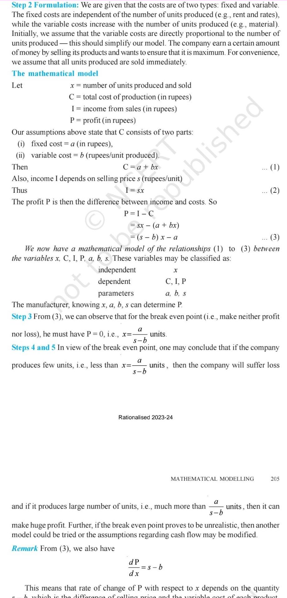
Permutations and CombinationsStep 2 Formulation We are given that the costs are of two types fixed and variable The fixed costs are independent of the number of units produced e g rent and rates while the variable costs increase with the number of units produced e g material Initially we assume that the variable costs are directly proportional to the number of units produced this should simplify our model The company earn a certain amount of money by selling its products and wants to ensure that it is maximum For convenience we assume that all units produced are sold immediately The mathematical model Let x number of units produced and sold C total cost of production in rupees I income from sales in rupees P profit in rupees Our assumptions above state that C consists of two parts i fixed cost a in rupees ii variable cost b rupees unit produced Then C a bx Also income I depends on selling price s rupees uni Thus I Sx The profit P is then the difference between income and costs So s b x a independent dependent 3 We now have a mathematical model of the relationships 1 to 3 between the variables x C I P a b s These variables may be classified as Rationalised 2023 24 ot to be published X C I P parameters a b s The manufacturer knowing x a b s can determine P Step 3 From 3 we can observe that for the break even point i e make neither profit a nor loss he must have P 0 i e x units s b Steps 4 and 5 In view of the break even point one may conclude that if the company produces few units i e less than x units then the company will suffer loss s b a dP dx 1 s b MATHEMATICAL MODELLING a s b and if it produces large number of units i e much more than units then it can make huge profit Further if the break even point proves to be unrealistic then another model could be tried or the assumptions regarding cash flow may be modified Remark From 3 we also have 205 This means that rate of change of P with respect to x depends on the quantity h which is the difference of selling price and the variable cost of each product
Algebra
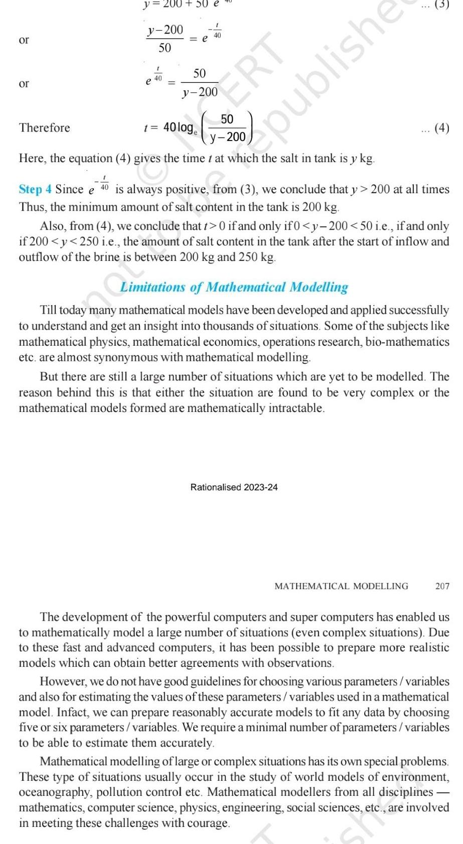
Complex numbersor or y 200 50 e y 200 50 Therefore 40 e 1 50 40 ERT 40 loge Here the equation 4 gives the time t at which the salt in tank is y kg Step 4 Since e 40 is always positive from 3 we conclude that y 200 at all times Thus the minimum amount of salt content in the tank is 200 kg publishe 3 Also from 4 we conclude that t 0 if and only if 0 y 200 50 i e if and only if 200 y 250 i e the amount of salt content in the tank after the start of inflow and outflow of the brine is between 200 kg and 250 kg Rationalised 2023 24 4 Limitations of Mathematical Modelling Till today many mathematical models have been developed and applied successfully to understand and get an insight into thousands of situations Some of the subjects like mathematical physics mathematical economics operations research bio mathematics etc are almost synonymous with mathematical modelling But there are still a large number of situations which are yet to be modelled The reason behind this is that either the situation are found to be very complex or the mathematical models formed are mathematically intractable MATHEMATICAL MODELLING 207 The development of the powerful computers and super computers has enabled us to mathematically model a large number of situations even complex situations Due to these fast and advanced computers it has been possible to prepare more realistic models which can obtain better agreements with observations However we do not have good guidelines for choosing various parameters variables and also for estimating the values of these parameters variables used in a mathematical model Infact we can prepare reasonably accurate models to fit any data by choosing five or six parameters variables We require a minimal number of parameters variables to be able to estimate them accurately Mathematical modelling of large or complex situations has its own special problems These type of situations usually occur in the study of world models of environment oceanography pollution control etc Mathematical modellers from all disciplines mathematics computer science physics engineering social sciences are involved in meeting these challenges with courage
Algebra
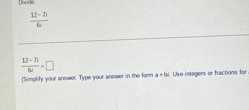
Complex numbersDivide 12 7i 6i 12 7i 6i Simplify your answer Type your answer in the form a bi Use integers or fractions for
Algebra
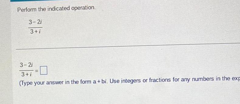
Complex numbersPerform the indicated operation 3 2i 3 i 3 2i 3 i Type your answer in the form a bi Use integers or fractions for any numbers in the exp
Algebra
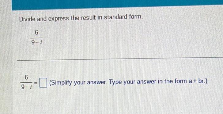
Quadratic equationsDivide and express the result in standard form 6 9 i 6 9 i Simplify your answer Type your answer in the form a bi
Algebra
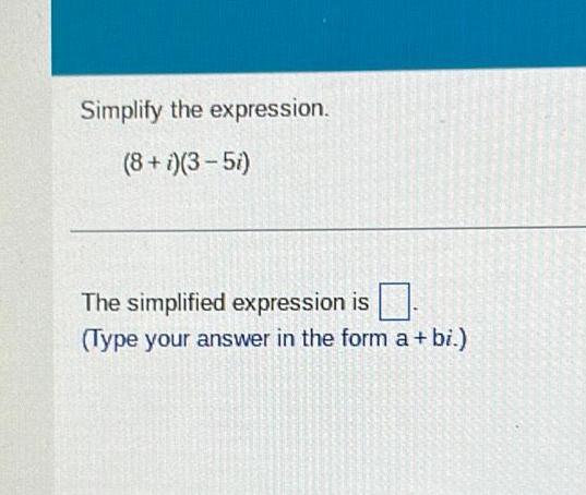
Quadratic equationsSimplify the expression 8 i 3 5i The simplified expression is Type your answer in the form a bi
Algebra
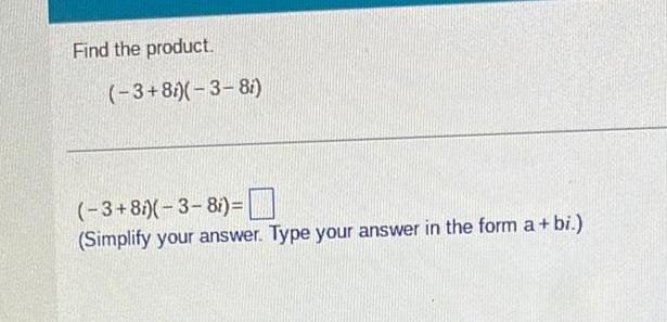
Complex numbersFind the product 3 8i 3 8i 3 8i 3 8 Simplify your answer Type your answer in the form a bi
Algebra
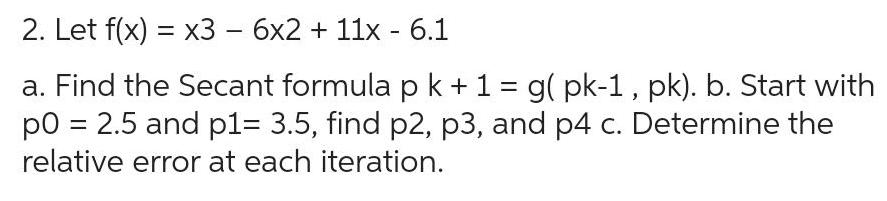
Sequences & Series2 Let f x x3 6x2 11x 6 1 a Find the Secant formula p k 1 g pk 1 pk b Start with p0 2 5 and p1 3 5 find p2 p3 and p4 c Determine the relative error at each iteration
Algebra
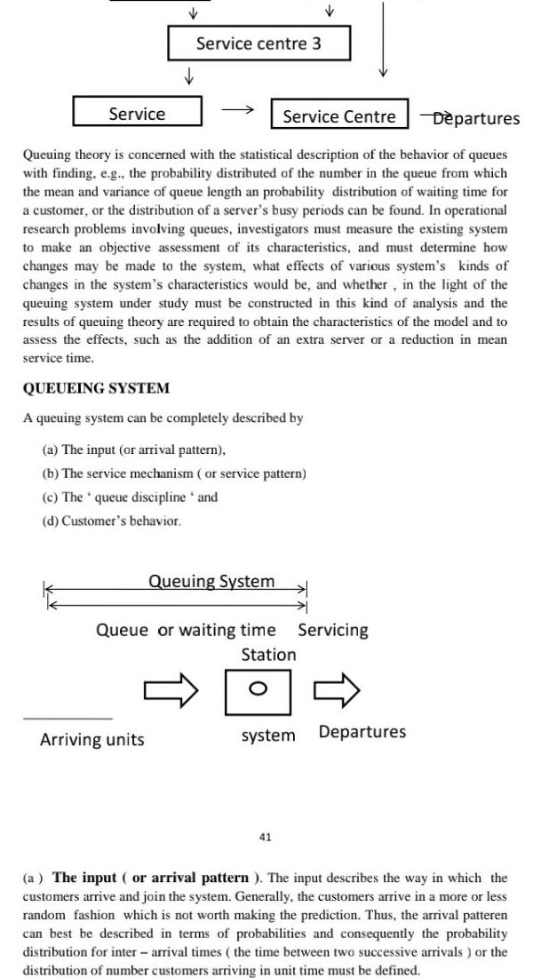
Quadratic equationsService Service centre 3 Departures Queuing theory is concerned with the statistical description of the behavior of queues with finding e g the probability distributed of the number in the queue from which the mean and variance of queue length an probability distribution of waiting time for a customer or the distribution of a server s busy periods can be found In operational research problems involving queues investigators must measure the existing system to make an objective assessment of its characteristics and must determine how changes may be made to the system what effects of various system s kinds of changes in the system s characteristics would be and whether in the light of the queuing system under study must be constructed in this kind of analysis and the results of queuing theory are required to obtain the characteristics of the model and to assess the effects such as the addition of an extra server or a reduction in mean service time Arriving units QUEUEING SYSTEM A queuing system can be completely described by a The input or arrival pattern b The service mechanism or service pattern c The queue discipline and d Customer s behavior Queuing System Service Centre Queue or waiting time Servicing Station 0 41 system Departures a The input or arrival pattern The input describes the way in which the customers arrive and join the system Generally the customers arrive in a more or less random fashion which is not worth making the prediction Thus the arrival patteren can best be described in terms of probabilities and consequently the probability distribution for inter arrival times the time between two successive arrivals or the distribution of number customers arriving in unit time must be defined
Algebra
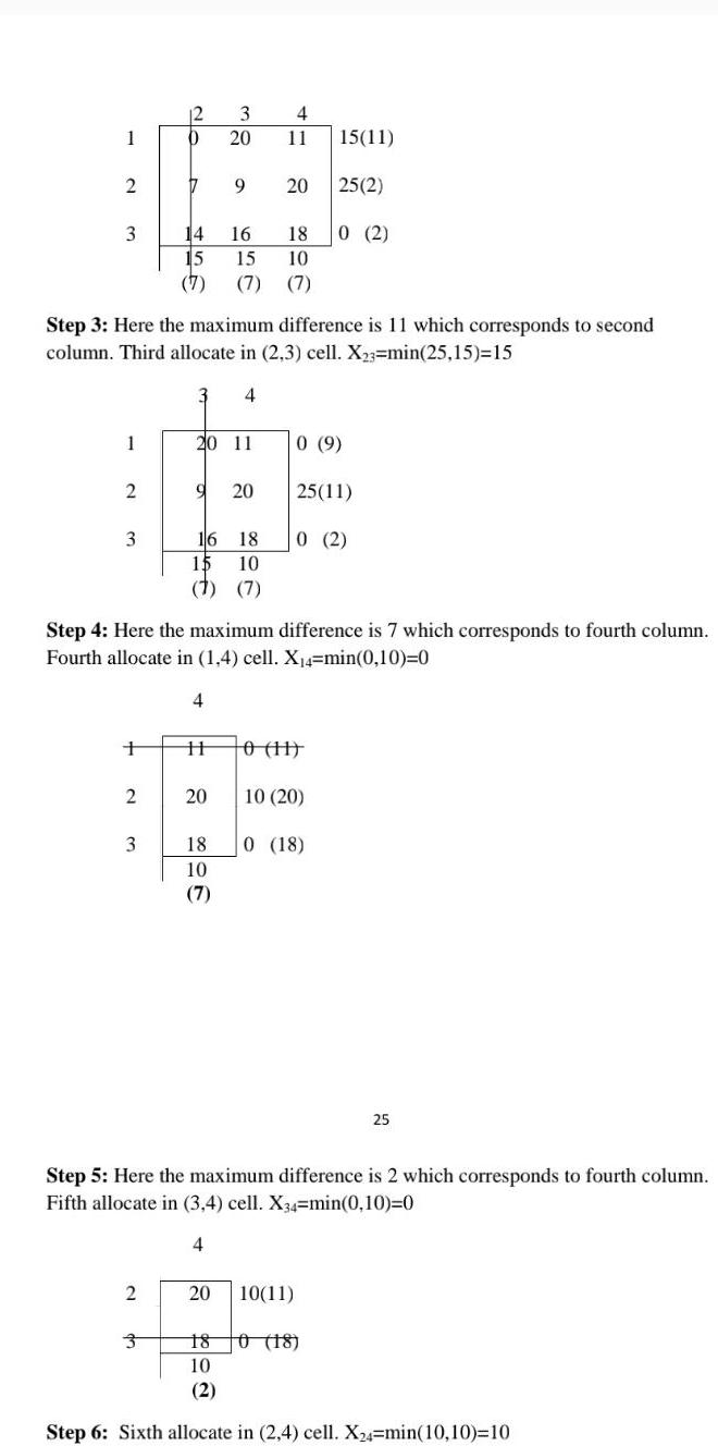
Complex numbers1 2 3 1 2 3 2 3 12 3 0 20 Step 3 Here the maximum difference is 11 which corresponds to second column Third allocate in 2 3 cell X 3 min 25 15 15 3 4 17 9 2 3 14 16 15 15 10 7 7 7 16 18 15 10 7 7 4 11 20 Step 4 Here the maximum difference is 7 which corresponds to fourth column Fourth allocate in 1 4 cell X 4 min 0 10 0 4 20 20 11 0 9 9 20 18 10 7 18 0 2 15 11 25 2 H 0 11 10 20 25 11 0 2 20 10 11 0 18 Step 5 Here the maximum difference is 2 which corresponds to fourth column Fifth allocate in 3 4 cell X34 min 0 10 0 4 25 18 0 18 10 2 Step 6 Sixth allocate in 2 4 cell X24 min 10 10 10
Algebra
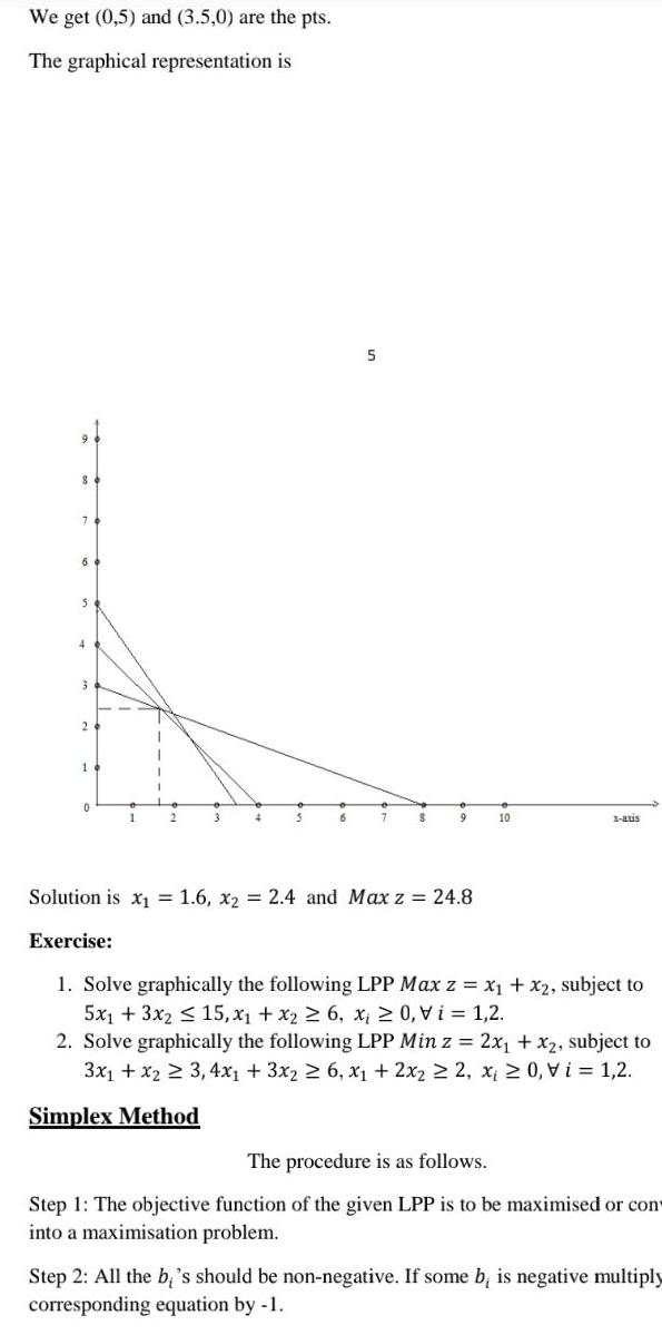
Quadratic equationsWe get 0 5 and 3 5 0 are the pts The graphical representation is 3 6 5 S 9 10 1 aus Solution is x 1 6 x 2 4 and Max z 24 8 Exercise 1 Solve graphically the following LPP Max z x x2 subject to 5x1 3x2 15 x x 6 x 0 Vi 1 2 2 Solve graphically the following LPP Min z 2x x2 subject to 3x1 x2 3 4x 3x 6 x 2x 2 x 0 Vi 1 2 Simplex Method The procedure is as follows Step 1 The objective function of the given LPP is to be maximised or con into a maximisation problem Step 2 All the bi s should be non negative If some b is negative multiply corresponding equation by 1
Algebra
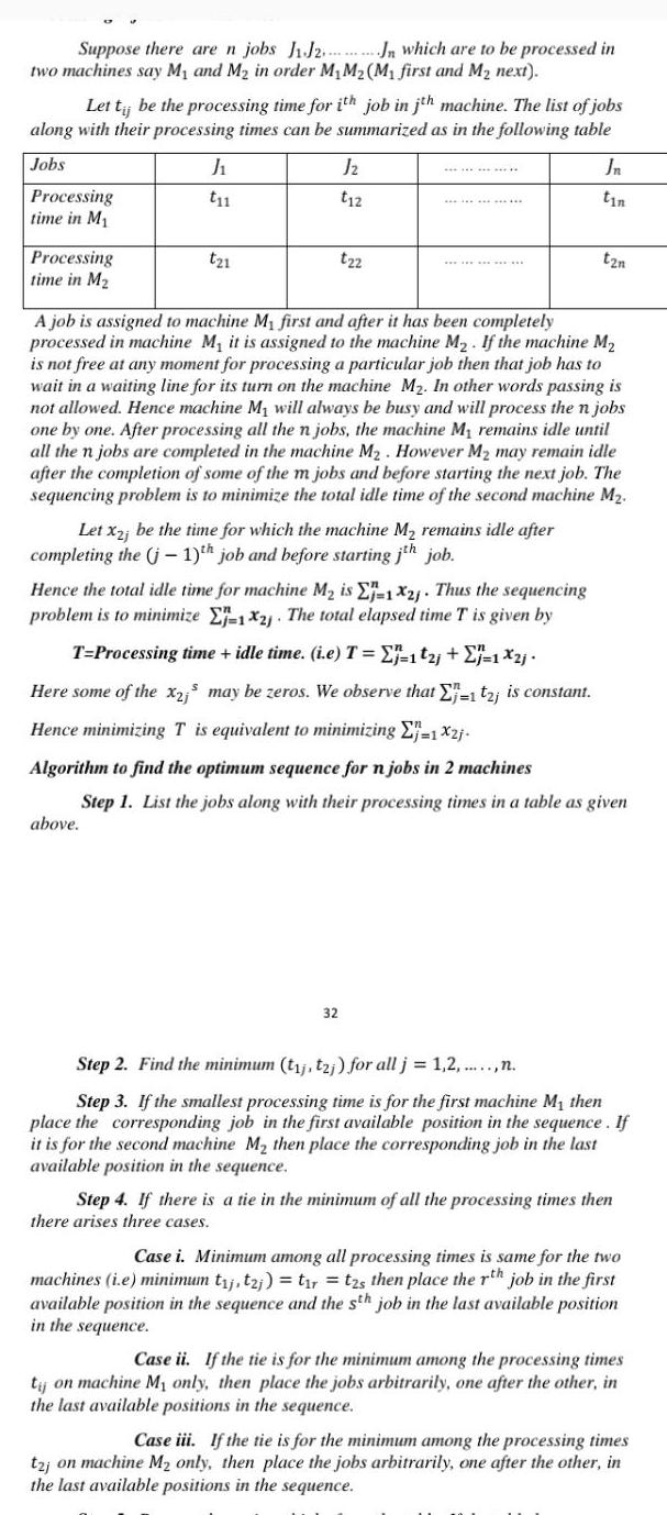
Complex numbersSuppose there are n jobs J1 J2 two machines say M and M in order M M M first and M next Let t be the processing time for ith job in jth machine The list of jobs along with their processing times can be summarized as in the following table Jobs Processing time in M Processing time in M J t11 t21 above Jn which are to be processed in Jz t12 t22 Let x2j be the time for which the machine M remains idle after completing the j 1 th job and before starting jth job A job is assigned to machine My first and after it has been completely processed in machine M it is assigned to the machine M If the machine M is not free at any moment for processing a particular job then that job has to wait in a waiting line for its turn on the machine M In other words passing is not allowed Hence machine M will always be busy and will process the n jobs one by one After processing all the n jobs the machine M remains idle until all the n jobs are completed in the machine M However M may remain idle after the completion of some of the m jobs and before starting the next job The sequencing problem is to minimize the total idle time of the second machine M 32 Jn tin tzn Hence the total idle time for machine M is E 1X2j Thus the sequencing problem is to minimize E 12 The total elapsed time T is given by T Processing time idle time i e T j 121 1 2 Here some of the x2 may be zeros We observe that E 1 t2j is constant Hence minimizing T is equivalent to minimizing 1x2j Algorithm to find the optimum sequence for n jobs in 2 machines Step 1 List the jobs along with their processing times in a table as given Step 2 Find the minimum t j tzj for all j 1 2 n Step 3 If the smallest processing time is for the first machine M then place the corresponding job in the first available position in the sequence If it is for the second machine M then place the corresponding job in the last available position in the sequence Step 4 If there is a tie in the minimum of all the processing times then there arises three cases Case i Minimum among all processing times is same for the two machines i e minimum t j tzj t r tzs then place the rth job in the first available position in the sequence and the sth job in the last available position in the sequence Case it If the tie is for the minimum among the processing times tij on machine My only then place the jobs arbitrarily one after the other in the last available positions in the sequence Case iii If the tie is for the minimum among the processing times t2j on machine M only then place the jobs arbitrarily one after the other in the last available positions in the sequence