Statistics Questions
The best high school and college tutors are just a click away, 24×7! Pick a subject, ask a question, and get a detailed, handwritten solution personalized for you in minutes. We cover Math, Physics, Chemistry & Biology.
Statistics
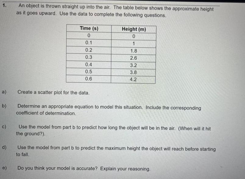
Probability1 a b c d e An object is thrown straight up into the air The table below shows the approximate height as it goes upward Use the data to complete the following questions Time s 0 0 1 0 2 0 3 0 4 0 5 0 6 Height m 0 1 1 8 2 6 3 2 3 8 4 2 Create a scatter plot for the data Determine an appropriate equation to model this situation Include the corresponding coefficient of determination Use the model from part b to predict how long the object will be in the air When will it hit the ground Use the model from part b to predict the maximum height the object will reach before starting to fall Do you think your model is accurate Explain your reasoning
Statistics
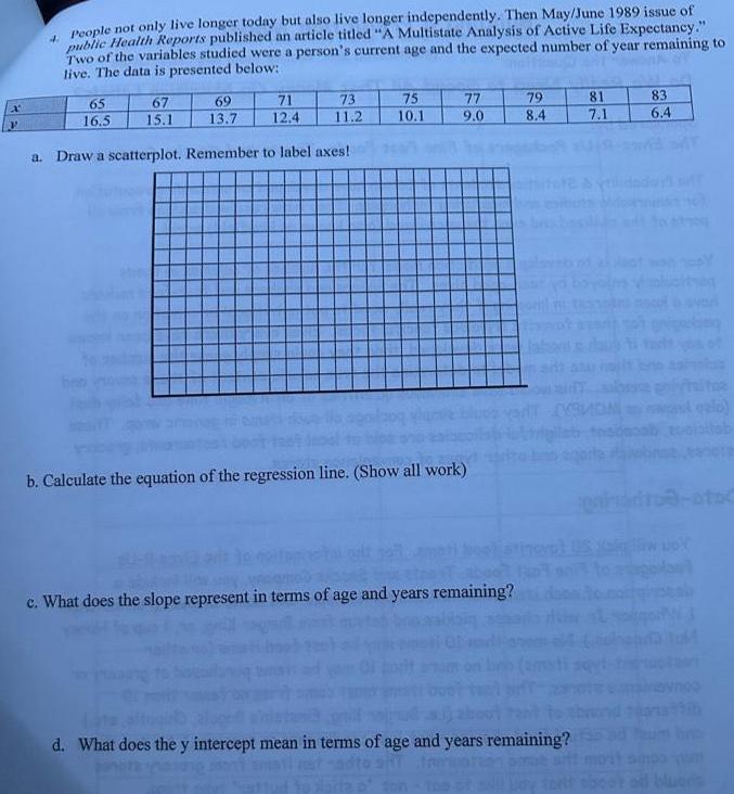
Statistics4 People not only live longer today but also live longer independently Then May June 1989 issue of public Health Reports published an article titled A Multistate Analysis of Active Life Expectancy Two of the variables studied were a person s current age and the expected number of year remaining to live The data is presented below 65 16 5 67 15 1 69 13 7 73 11 2 71 12 4 a Draw a scatterplot Remember to label axes 75 10 1 77 9 0 b Calculate the equation of the regression line Show all work c What does the slope represent in terms of age and years remaining 79 8 4 d What does the y intercept mean in terms of age and years remaining 81 7 1 83 6 4 tort sboot od bluoris
Statistics
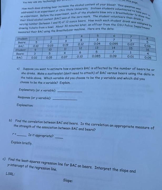
StatisticsThis page You may use any technology oddressed in an experiment at Ohio State University Sixteen students volunteered to take part in How much does drinking beer increase the alcohol content of your blood This question was an experiment Before the experiment each of the students blew into a Breathalyzer to show that their blood alcohol content BAC was at the zero mark The student volunteers then drank a varying number between 1 and 9 of 12 ounce beers How much each student drank was assigned by drawing tickets from a bowl About 30 minutes later an officer from the OSU Police Department measured their BAC using the Breathalyzer machine Here are the data Student Beers BAC Student Beers BAC r 1 5 0 10 9 3 0 02 Explain briefly 2 2 0 03 10 5 0 05 3 9 0 19 11 4 0 07 4 8 0 12 12 6 0 10 5 Slope 3 0 04 13 5 0 085 6 7 0 095 14 7 0 09 7 3 0 07 15 1 0 01 8 a Suppose you want to estimate how a person s BAC is affected by the number of beers he or she drinks Make a scatterplot don t need to attach of BAC versus beers using the data in the table above Which variable did you choose to be the y variable and which did you choose to be the x variable Explain Explanatory or x variable Response or y variable Explanation b Find the correlation between BAC and beers Is the correlation an appropriate measure of the strength of the association between BAC and beers Is it appropriate c Find the least squares regression line for BAC on beers Interpret the slope and y intercept of the regression line LSRL 5 0 06 16 4 0 05
Statistics
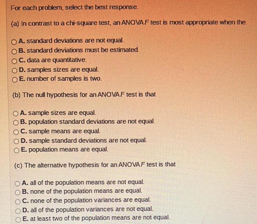
StatisticsFor each problem select the best response a In contrast to a chi square test an ANOVAF test is most appropriate when the A standard deviations are not equal OB standard deviations must be estimated OC data are quantitative OD samples sizes are equal E number of samples is two b The null hypothesis for an ANOVAF test is that OA sample sizes are equal OB population standard deviations are not equal OC sample means are equal OD sample standard deviations are not equal O E population means are equal c The alternative hypothesis for an ANOVAF test is that OA all of the population means are not equal OB none of the population means are equal OC none of the population variances are equal OD all of the population variances are not equal E at least two of the population means are not equal
Statistics
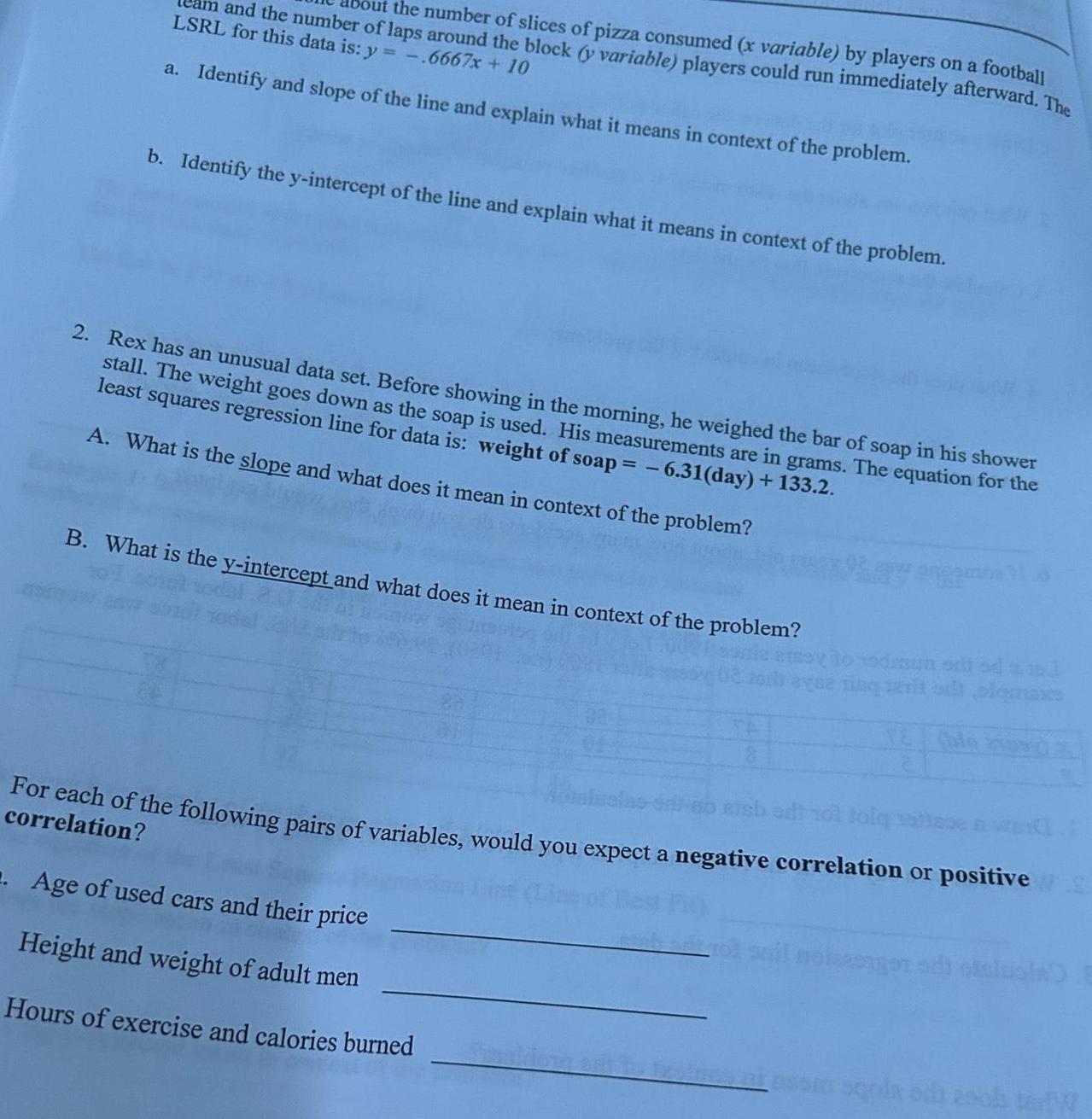
Statisticsand the number of laps around the block y variable players could run immediately afterward The the number of slices of pizza consumed x variable by players on a football LSRL for this data is y 6667x 10 a Identify and slope of the line and explain what it means in context of the problem b Identify the y intercept of the line and explain what it means in context of the problem 2 Rex has an unusual data set Before showing in the morning he weighed the bar of soap in his shower stall The weight goes down as the soap is used His measurements are in grams The equation for the least squares regression line for data is weight of soap 6 31 day 133 2 A What is the slope and what does it mean in context of the problem B What is the y intercept and what does it mean in context of the problem 19dum odi zad For each of the following pairs of variables would you expect a negative correlation or positive S correlation 2 Age of used cars and their price Height and weight of adult men Hours of exercise and calories burned
Statistics
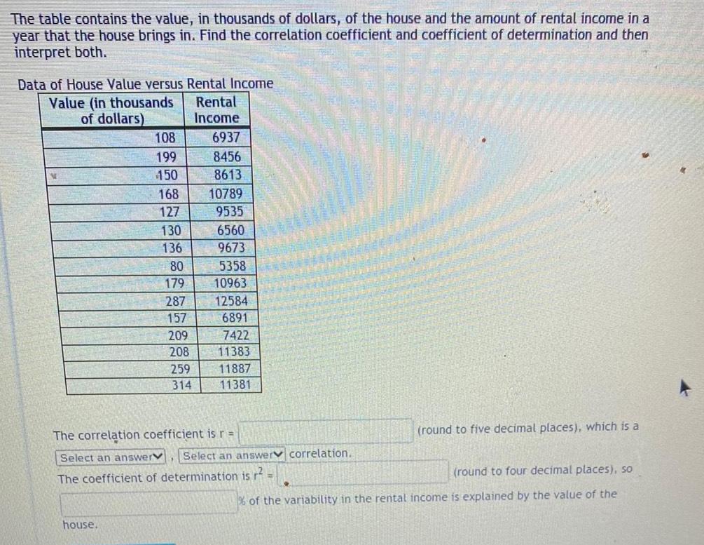
StatisticsThe table contains the value in thousands of dollars of the house and the amount of rental income in a year that the house brings in Find the correlation coefficient and coefficient of determination and then interpret both Data of House Value versus Rental Income Value in thousands Rental of dollars Income 108 199 150 house 168 127 130 136 80 179 287 157 209 208 259 314 6937 8456 8613 10789 9535 6560 9673 5358 10963 12584 6891 7422 11383 11887 11381 MA The correlation coefficient is r Select an answerv Select an answer correlation The coefficient of determination is r round to five decimal places which is a round to four decimal places so of the variability in the rental income is explained by the value of the
Statistics
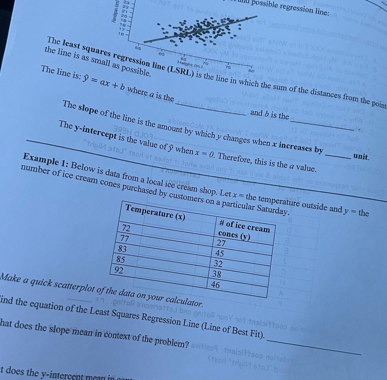
StatisticsHandspan cm ANNAPPER 19 18 17 16 60 65 70 75 80 The least squares regression line LSRL is the line in which the sum of the distances from the point is as as possible TAB The line is ax b where a is the not qot to svidanp 55 72 77 83 85 92 hondartla not wodlestol pea ainT striW of bill XXX amor bonHI A dribor xalqmo a loodbe doit vM 2 A 20 XXX YM to ygosotorio a sish peed A riti od of tor tIoT msagn The slope of the line is the amount by which y changes when x increases by a blonodom ta boxnow I narW boot of bid I epnir possible regression line otro basta t does the y intercept mean in cont spalloa ni noitastiA 393H OJO The y intercept is the value of when x 0 Therefore this is the a value trei stoj teori of 29xpt ti toriw svorl upyti ssa ll sw sidot silt no esenogean musy sund Example 1 Below is data from a local ice cream shop Let x the temperature outside and y the number of ice cream cones purchased by customers on a particular Saturday Temperature x and b is the 27 45 of ice cream cones y 32 38 46 Make a quick scatterplot of the data on your calculator ind the equation of the Least Squares Regression Line Line of Best Fit enito anomstts bro gritos nuoY not tnsisittsos noitph That does the slope mean in context of the problem svitizo9 tasisittsos noitels Steor tripi stol boog 22073 unit 3934 000
Statistics
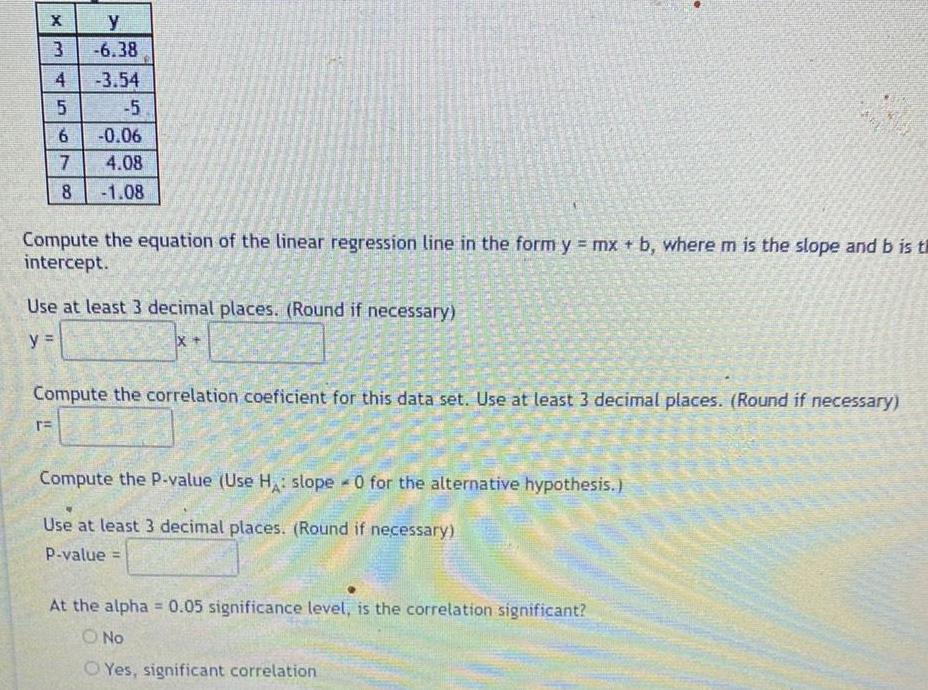
Probabilityy 3 6 38 3 54 5 6 0 06 7 4 08 8 1 08 EX 4 TE 45 Compute the equation of the linear regression line in the form y mx b where m is the slope and b is th intercept Use at least 3 decimal places Round if necessary y IX Compute the correlation coeficient for this data set Use at least 3 decimal places Round if necessary Compute the P value Use H slope 0 for the alternative hypothesis A Use at least 3 decimal places Round if necessary P value At the alpha 0 05 significance level is the correlation significant O No Yes significant correlation
Statistics
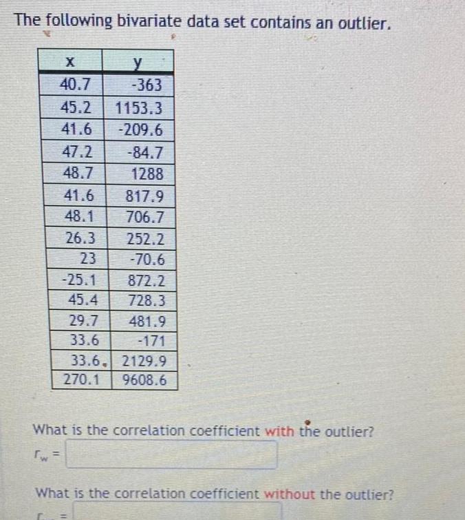
StatisticsThe following bivariate data set contains an outlier X 40 7 45 2 1153 3 41 6 209 6 47 2 48 7 41 6 48 1 26 3 25 1 45 4 29 7 33 6 33 6 270 1 y 363 84 7 1288 817 9 706 7 252 2 70 6 872 2 728 3 481 9 2129 9 9608 6 What is the correlation coefficient with the outlier w What is the correlation coefficient without the outlier
Statistics
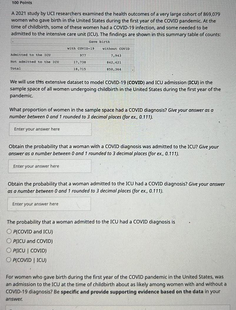
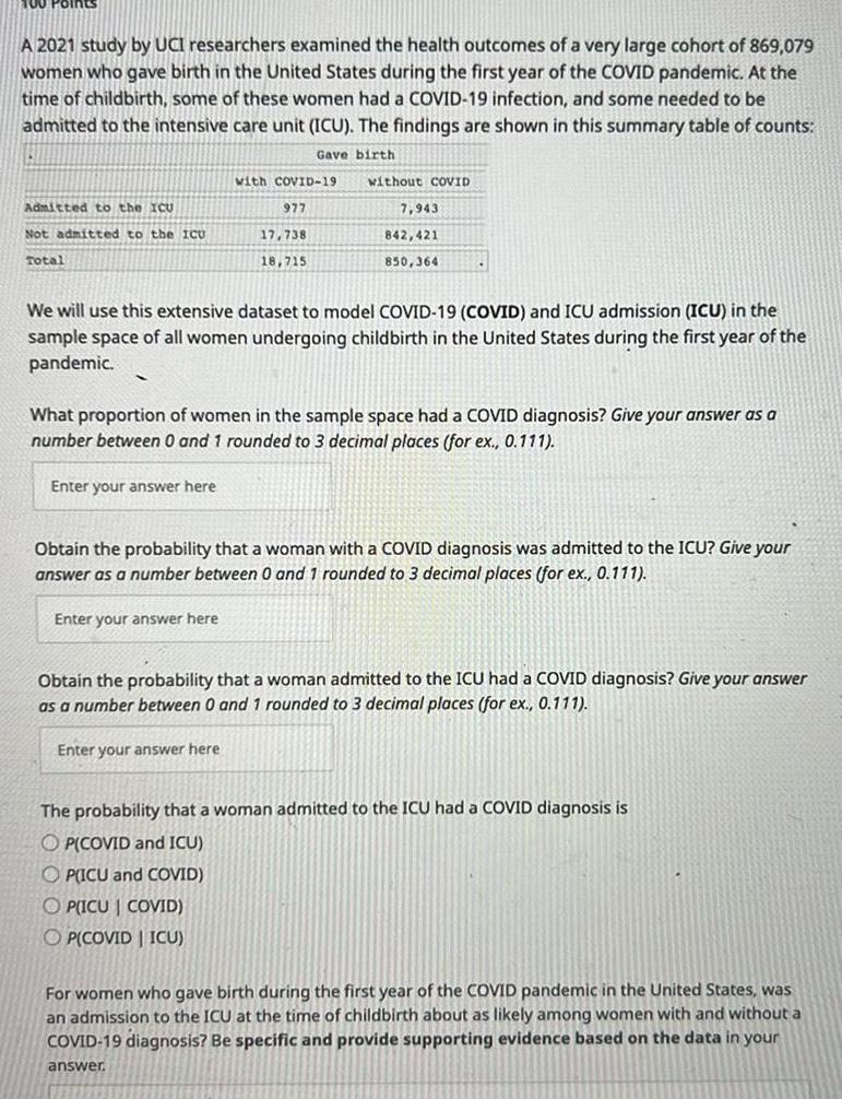
Probability100 Points A 2021 study by UCI researchers examined the health outcomes of a very large cohort of 869 079 women who gave birth in the United States during the first year of the COVID pandemic At the time of childbirth some of these women had a COVID 19 infection and some needed to be admitted to the intensive care unit ICU The findings are shown in this summary table of counts Gave birth Admitted to the ICU Not admitted to the ICU Total with COVID 19 Enter your answer here 977 17 738 18 715 without coVID We will use this extensive dataset to model COVID 19 COVID and ICU admission ICU in the sample space of all women undergoing childbirth in the United States during the first year of the pandemic Enter your answer here 7 943 842 421 850 364 What proportion of women in the sample space had a COVID diagnosis Give your answer as a number between 0 and 1 rounded to 3 decimal places for ex 0 111 Obtain the probability that a woman with a COVID diagnosis was admitted to the ICU Give your answer as a number between 0 and 1 rounded to 3 decimal places for ex 0 111 Enter your answer here Obtain the probability that a woman admitted to the ICU had a COVID diagnosis Give your answer as a number between 0 and 1 rounded to 3 decimal places for ex 0 111 The probability that a woman admitted to the ICU had a COVID diagnosis is OP COVID and ICU OP ICU and COVID P ICU COVID PICOVIDICU For women who gave birth during the first year of the COVID pandemic in the United States was an admission to the ICU at the time of childbirth about as likely among women with and without a COVID 19 diagnosis Be specific and provide supporting evidence based on the data in your answer
Statistics
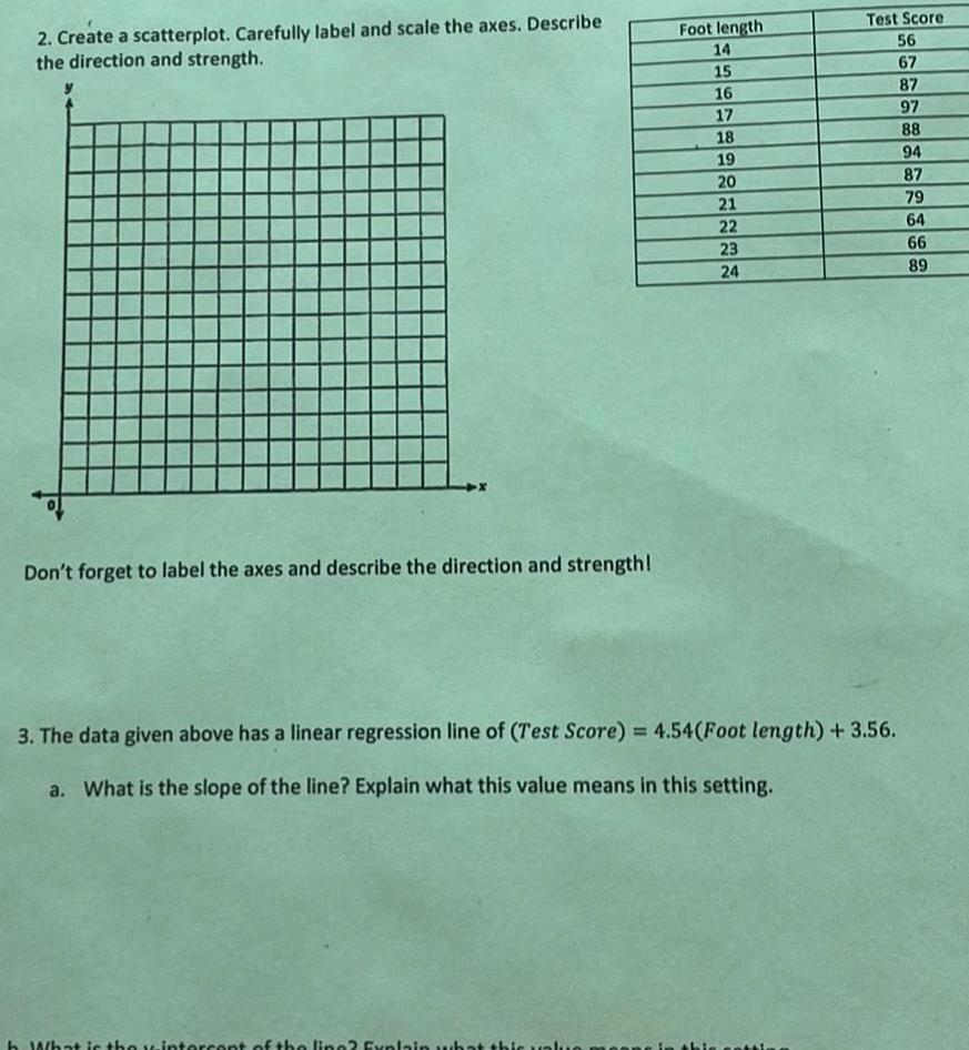
Statistics2 Create a scatterplot Carefully label and scale the axes Describe the direction and strength Don t forget to label the axes and describe the direction and strength Foot length 14 15 16 17 18 19 20 21 22 23 24 h What is the wintercent of the line Explain what thic value 3 The data given above has a linear regression line of Test Score 4 54 Foot length 3 56 a What is the slope of the line Explain what this value means in this setting Test Score 56 67 setti 87 97 88 94 87 79 64 66 89
Statistics
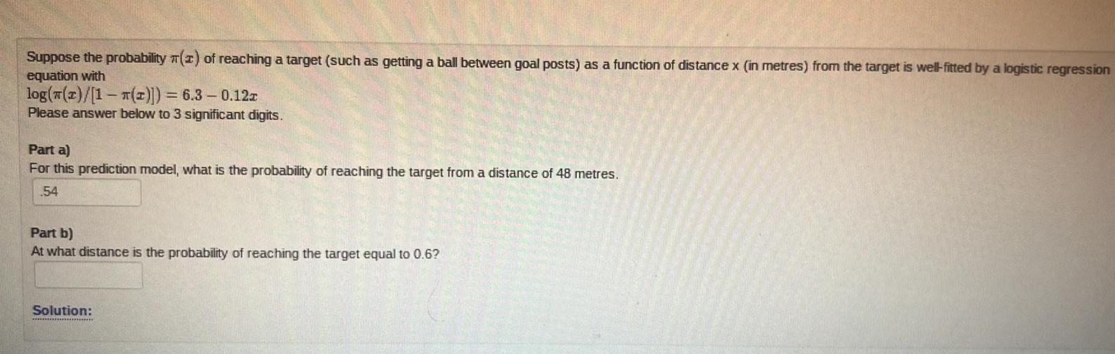
StatisticsSuppose the probability 2 of reaching a target such as getting a ball between goal posts as a function of distance x in metres from the target is well fitted by a logistic regression equation with log z 1 2 6 3 0 12x Please answer below to 3 significant digits Part a For this prediction model what is the probability of reaching the target from a distance of 48 metres 54 Part b At what distance is the probability of reaching the target equal to 0 6 Solution
Statistics
ProbabilityA 2021 study by UCI researchers examined the health outcomes of a very large cohort of 869 079 women who gave birth in the United States during the first year of the COVID pandemic At the time of childbirth some of these women had a COVID 19 infection and some needed to be admitted to the intensive care unit ICU The findings are shown in this summary table of counts Gave birth Admitted to the ICU Not admitted to the ICU Total with COVID 19 977 Enter your answer here 17 738 18 715 without COVID 7 943 842 421 850 364 We will use this extensive dataset to model COVID 19 COVID and ICU admission ICU in the sample space of all women undergoing childbirth in the United States during the first year of the pandemic What proportion of women in the sample space had a COVID diagnosis Give your answer as a number between 0 and 1 rounded to 3 decimal places for ex 0 111 Obtain the probability that a woman with a COVID diagnosis was admitted to the ICU Give your answer as a number between 0 and 1 rounded to 3 decimal places for ex 0 111 Enter your answer here Obtain the probability that a woman admitted to the ICU had a COVID diagnosis Give your answer as a number between 0 and 1 rounded to 3 decimal places for ex 0 111 Enter your answer here The probability that a woman admitted to the ICU had a COVID diagnosis is OP COVID and ICU OP ICU and COVID OPICU COVID OP COVID ICU For women who gave birth during the first year of the COVID pandemic in the United States was an admission to the ICU at the time of childbirth about as likely among women with and without a COVID 19 diagnosis Be specific and provide supporting evidence based on the data in your answer
Statistics
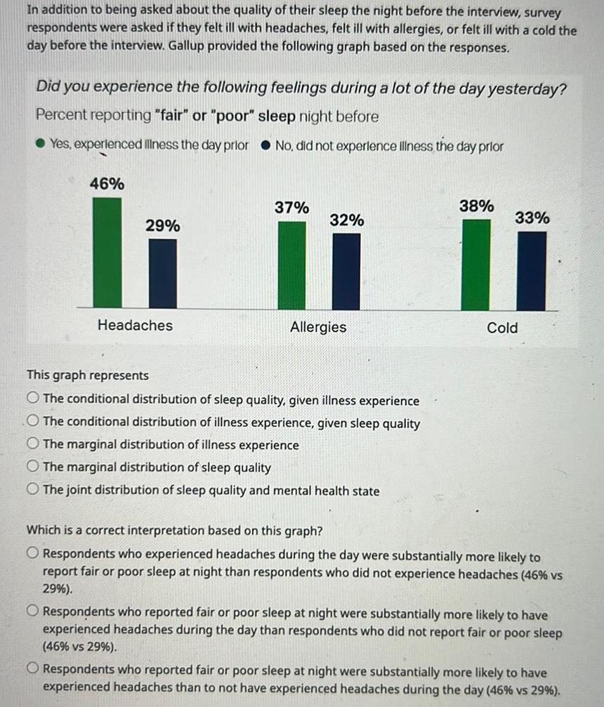
StatisticsIn addition to being asked about the quality of their sleep the night before the interview survey respondents were asked if they felt ill with headaches felt ill with allergies or felt ill with a cold the day before the interview Gallup provided the following graph based on the responses Did you experience the following feelings during a lot of the day yesterday Percent reporting fair or poor sleep night before Yes experienced illness the day prior No did not experience illness the day prior 46 29 Headaches 37 32 Allergies This graph represents O The conditional distribution of sleep quality given illness experience O The conditional distribution of illness experience given sleep quality O The marginal distribution of illness experience The marginal distribution of sleep quality The joint distribution of sleep quality and mental health state 38 33 Cold Which is a correct interpretation based on this graph O Respondents who experienced headaches during the day were substantially more likely to report fair or poor sleep at night than respondents who did not experience headaches 46 vs 29 O Respondents who reported fair or poor sle night were substantially more likely to have experienced headaches during the day than respondents who did not report fair or poor sleep 46 vs 29 O Respondents who reported fair or poor sleep at night were substantially more likely to have experienced headaches than to not have experienced headaches during the day 46 vs 29
Statistics
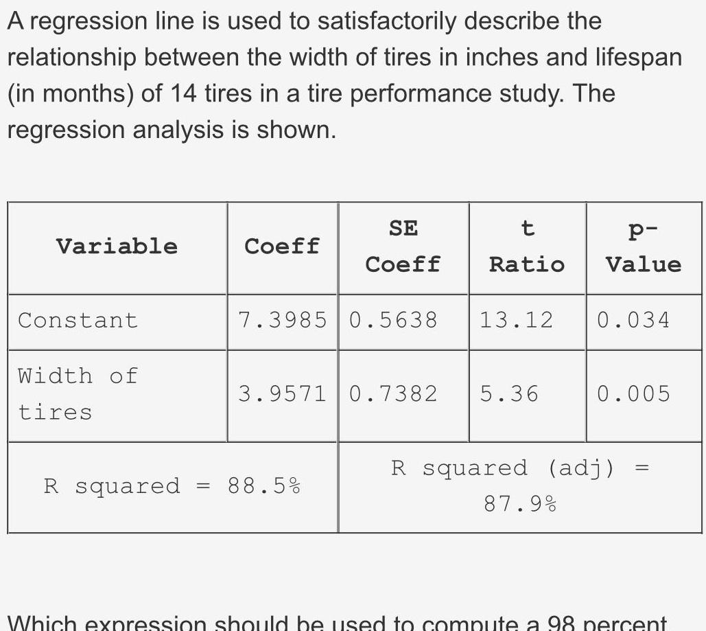
StatisticsA regression line is used to satisfactorily describe the relationship between the width of tires in inches and lifespan in months of 14 tires in a tire performance study The regression analysis is shown Variable Constant Width of tires R squared Coeff SE Coeff t Ratio 88 5 7 3985 0 5638 13 12 0 034 3 9571 0 7382 5 36 p Value 87 9 0 005 R squared adj Which expression should be used to compute a 98 percent
Statistics
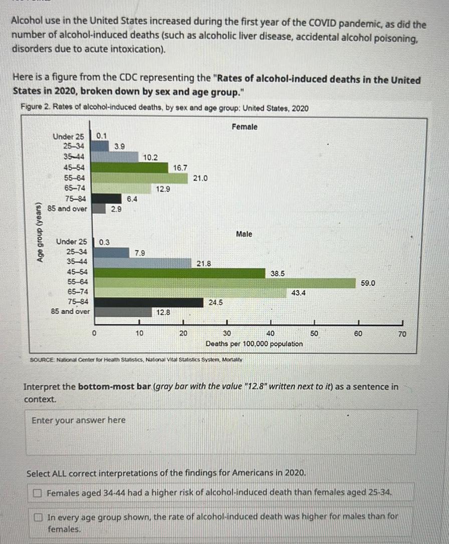
StatisticsAlcohol use in the United States increased during the first year of the COVID pandemic as did the number of alcohol induced deaths such as alcoholic liver disease accidental alcohol poisoning disorders due to acute intoxication Here is a figure from the CDC representing the Rates of alcohol induced deaths in the United States in 2020 broken down by sex and age group Figure 2 Rates of alcohol induced deaths by sex and age group United States 2020 Female Age group years Under 25 0 1 25 34 35 44 45 54 55 64 65 74 75 84 85 and over Under 25 25 34 35 44 45 54 55 64 65 74 75 84 85 and over 0 0 3 3 9 2 9 6 4 10 2 7 9 10 12 9 12 8 16 7 20 21 0 21 8 24 5 Male 38 5 SOURCE National Center for Health Statistics National Vital Statistics System Mortality I 30 Deaths per 100 000 population 43 4 40 50 59 0 I 60 Interpret the bottom most bar gray bar with the value 12 8 written next to it as a sentence in context Enter your answer here Select ALL correct interpretations of the findings for Americans in 2020 Females aged 34 44 had a higher risk of alcohol induced death than females aged 25 34 70 In every age group shown the rate of alcohol induced death was higher for males than for females
Statistics
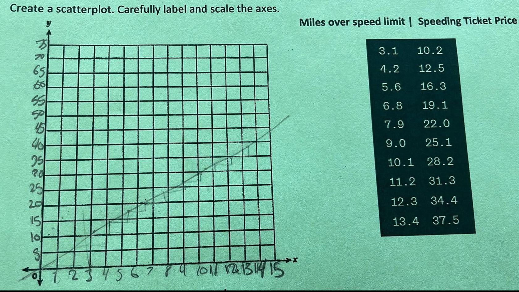
StatisticsCreate a scatterplot Carefully label and scale the axes 65 68 55 50 45 40 35 20 25 15 lo S 2 3 4 5 6 7 9 10 11 12 13 14 15 Miles over speed limit Speeding Ticket Price 3 1 10 2 4 2 12 5 5 6 16 3 6 8 19 1 7 9 22 0 9 0 25 1 10 1 28 2 11 2 31 3 12 3 34 4 13 4 37 5
Statistics
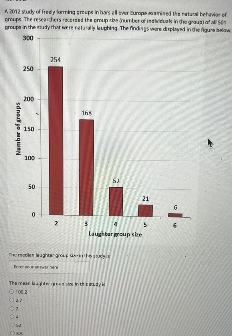
StatisticsA 2012 study of freely forming groups in bars all over Europe examined the natural behavior of groups The researchers recorded the group size number of individuals in the group of all 501 groups in the study that were naturally laughing The findings were displayed in the figure below 300 Number of groups 250 200 150 52 3 5 100 50 0 254 2 Enter your answer here 168 3 The median laughter group size in this study is The mean laughter group size in this study is 100 2 2 7 2 04 52 4 5 Laughter group size 21 6 6
Statistics
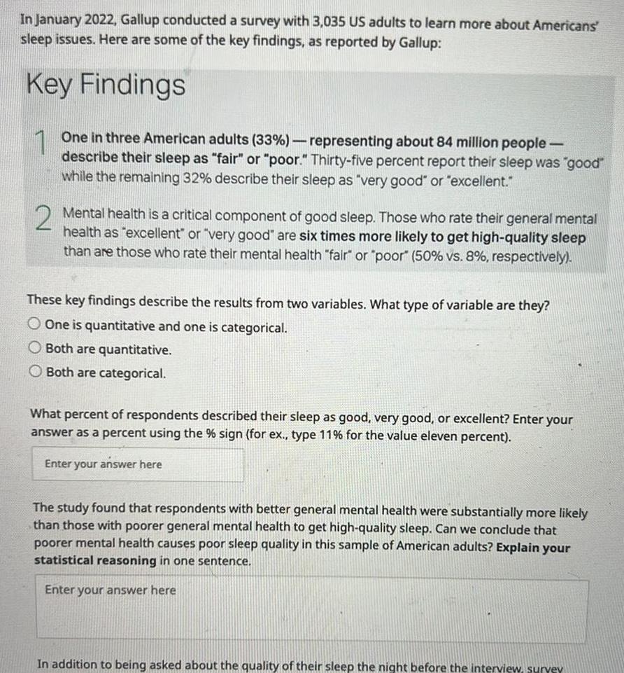
StatisticsIn January 2022 Gallup conducted a survey with 3 035 US adults to learn more about Americans sleep issues Here are some of the key findings as reported by Gallup Key Findings 1 One in three American adults 33 representing about 84 million people describe their sleep as fair or poor Thirty five percent report their sleep was good while the remaining 32 describe their sleep as very good or excellent 2 Mental health is a critical component of good sleep Those who rate their general mental health as excellent or very good are six times more likely to get high quality sleep than are those who rate their mental health fair or poor 50 vs 8 respectively These key findings describe the results from two variables What type of variable are they O One is quantitative and one is categorical O Both are quantitative O Both are categorical What percent of respondents described their sleep as good very good or excellent Enter your answer as a percent using the sign for ex type 11 for the value eleven percent Enter your answer here The study found that respondents with better general mental health were substantially more likely than those with poorer general mental health to get high quality sleep Can we conclude that poorer mental health causes poor sleep quality in this sample of American adults Explain your statistical reasoning in one sentence Enter your answer here In addition to being asked about the quality of their sleep the night before the interview survey
Statistics
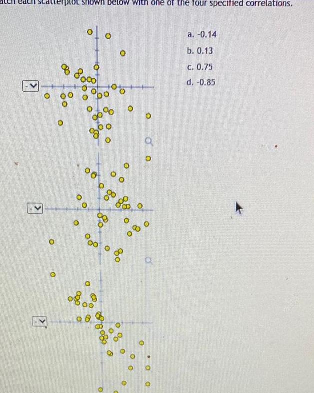
Probabilityach scatterplot shown below with one of the four specified correlations O O 8 8000 0 O 00 of o 0 0 00 00 00 08 0 00 O O O 80 O 00 O O 080 O Q O O Q O a 0 14 b 0 13 c 0 75 d 0 85
Statistics
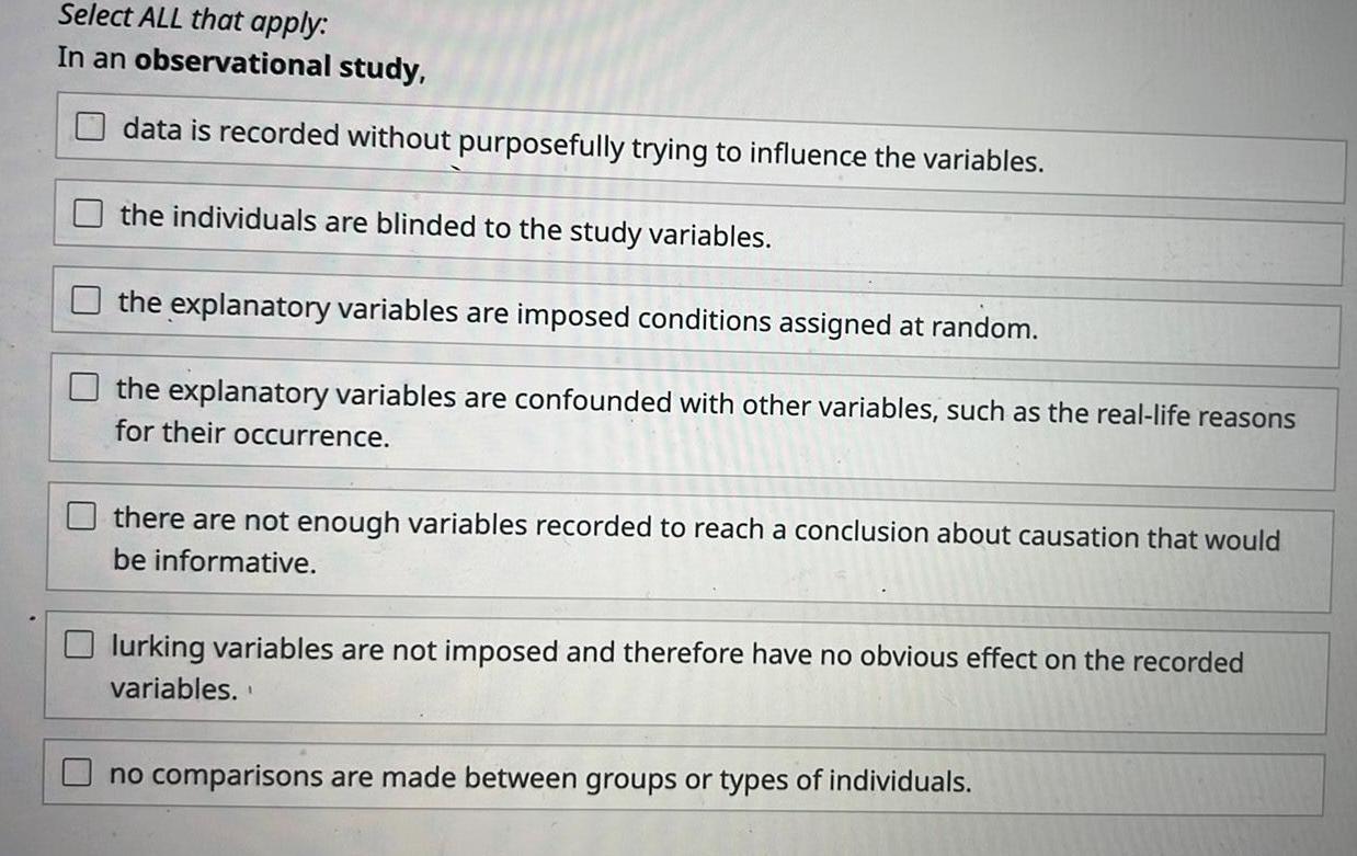
StatisticsSelect ALL that apply In an observational study data is recorded without purposefully trying to influence the variables the individuals are blinded to the study variables the explanatory variables are imposed conditions assigned at random the explanatory variables are confounded with other variables such as the real life reasons for their occurrence there are not enough variables recorded to reach a conclusion about causation that would be informative lurking variables are not imposed and therefore have no obvious effect on the recorded variables no comparisons are made between groups or types of individuals
Statistics
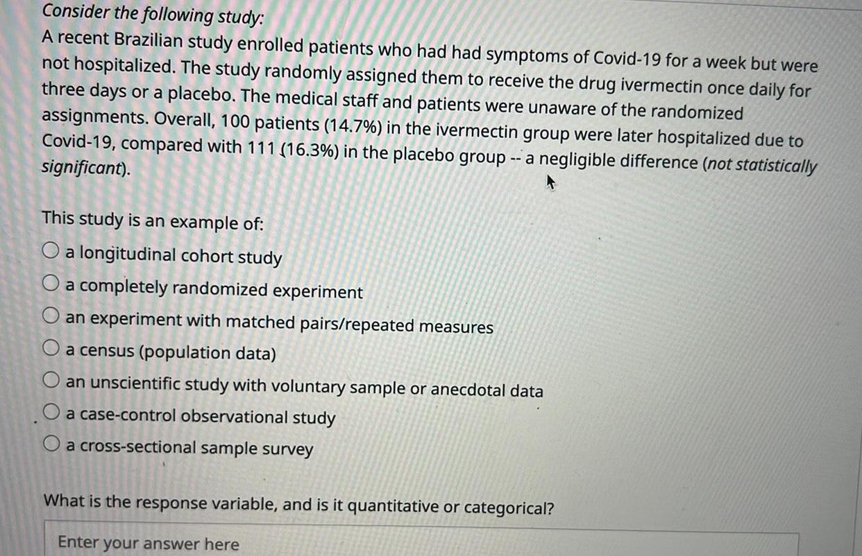
StatisticsConsider the following study A recent Brazilian study enrolled patients who had had symptoms of Covid 19 for a week but were not hospitalized The study randomly assigned them to receive the drug ivermectin once daily for three days or a placebo The medical staff and patients were unaware of the randomized assignments Overall 100 patients 14 7 in the ivermectin group were later hospitalized due to Covid 19 compared with 111 16 3 in the placebo group a negligible difference not statistically significant This study is an example of O a longitudinal cohort study a completely randomized experiment O an experiment with matched pairs repeated measures a census population data an unscientific study with voluntary sample or anecdotal data a case control observational study a cross sectional sample survey What is the response variable and is it quantitative or categorical Enter your answer here
Statistics
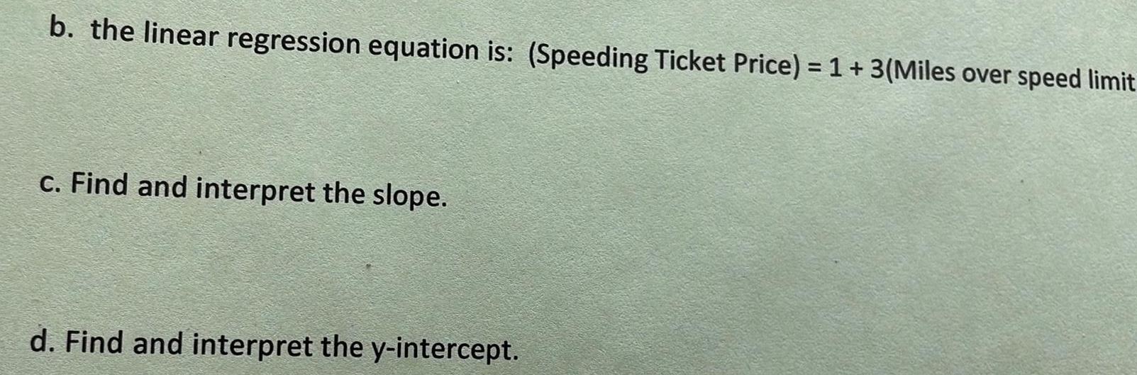
Statisticsb the linear regression equation is Speeding Ticket Price 1 3 Miles over speed limit c Find and interpret the slope d Find and interpret the y intercept
Statistics
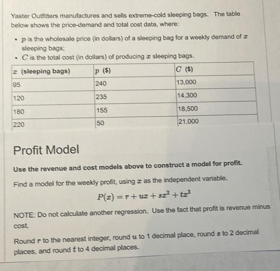
StatisticsYaster Outfitters manufactures and sells extreme cold sleeping bags The table below shows the price demand and total cost data where p is the wholesale price in dollars of a sleeping bag for a weekly demand of a sleeping bags C is the total cost in dollars of producing a sleeping bags sleeping bags C 13 000 14 300 18 500 21 000 120 220 240 235 155 50 Profit Model Use the revenue and cost models above to construct a model for profit Find a model for the weekly profit using z as the independent variable P z r uz sz tz NOTE Do not calculate another regression Use the fact that profit is revenue minus Round r to the nearest integer round us to 1 decimal place rounds to 2 decimal places and round t to 4 decimal places
Statistics
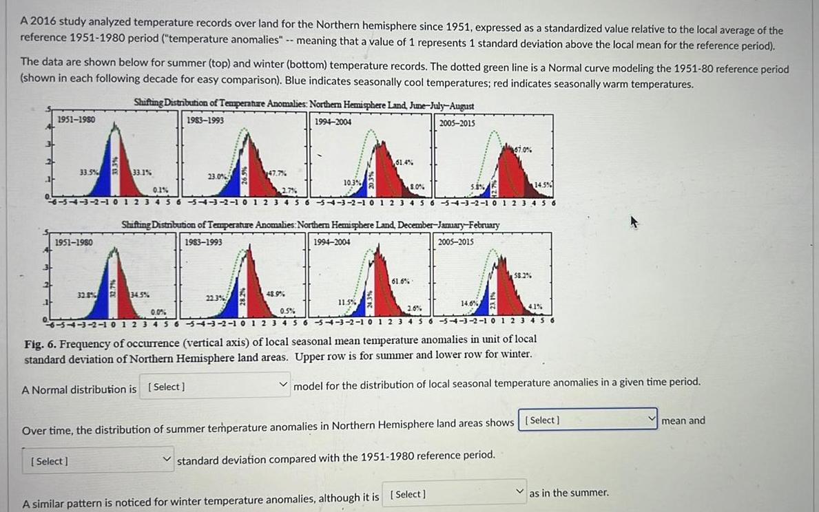
StatisticsA 2016 study analyzed temperature records over land for the Northern hemisphere since 1951 expressed as a standardized value relative to the local average of the reference 1951 1980 period temperature anomalies meaning that a value of 1 represents 1 standard deviation above the local mean for the reference period The data are shown below for summer top and winter bottom temperature records The dotted green line is a Normal curve modeling the 1951 80 reference period shown in each following decade for easy comparison Blue indicates seasonally cool temperatures red indicates seasonally warm temperatures 1951 1980 33 5 33 1 1951 1980 Shifting Distribution of Temperature Anomalies Northern Hemisphere Land June July August 1983 1993 1994 2004 Select 23 0 32 8 34 5 47 7 22 3 10 3 2 7 14 5 0 1 6 5 4 3 2 1 0 1 2 3 4 5 6 5 4 3 2 1 0 1 2 3 4 5 6 5 4 3 2 1 0 1 2 3 4 5 6 5 4 3 2 1 0 1 2 3 4 5 6 Shifting Distribution of Temperature Anomalies Northern Hemisphere Land December January February 1983 1993 2005 2015 48 9 1994 2004 61 4 11 5 8 0 61 6 2005 2015 5 8 67 0 14 6 A similar pattern is noticed for winter temperature anomalies although it is Select 2 6 4 1 0 0 0 5 6 54 3 2 1 0 1 2 3 4 5 6 5 4 3 2 1 0 1 2 3 4 5 6 5 4 3 2 1 0 1 2 3 4 5 6 5 4 3 2 1 0 1 2 3 4 5 6 Fig 6 Frequency of occurrence vertical axis of local seasonal mean temperature anomalies in unit of local standard deviation of Northern Hemisphere land areas Upper row is for summer and lower row for winter A Normal distribution is Select 58 2 model for the distribution of local seasonal temperature anomalies in a given time period Over time the distribution of summer temperature anomalies in Northern Hemisphere land areas shows Select standard deviation compared with the 1951 1980 reference period as in the summer mean and
Statistics
ProbabilityLet X be the cholesterol level in mg dl in the population of middle aged American men so that X follows the N 222 37 distribution The probability in this population of having borderline high cholesterol between 200 and 240 mg dl can be computed as Select In this population 90 of men have a cholesterol level that is at most Select mg dl V
Statistics
ProbabilityWhen a variable x is normally distributed the sampling distribution of the sample mean xbar O is correct O is also normally distributed O is uniformly distributed
Statistics
StatisticsWhy is the sample mean an unbiased estimator of the population mean O Because random samples are reliable O Because the mean of all sample means for random samples of the same size is equal to the mean of the entire population O Because populations are unbiased Because means are less variable than individual observations
Statistics
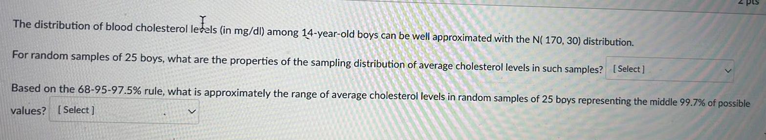
StatisticsI The distribution of blood cholesterol levels in mg dl among 14 year old boys can be well approximated with the N 170 30 distribution For random samples of 25 boys what are the properties of the sampling distribution of average cholesterol levels in such samples Select pts Based on the 68 95 97 5 rule what is approximately the range of average cholesterol levels in random samples of 25 boys representing the middle 99 7 of possible values Select
Statistics
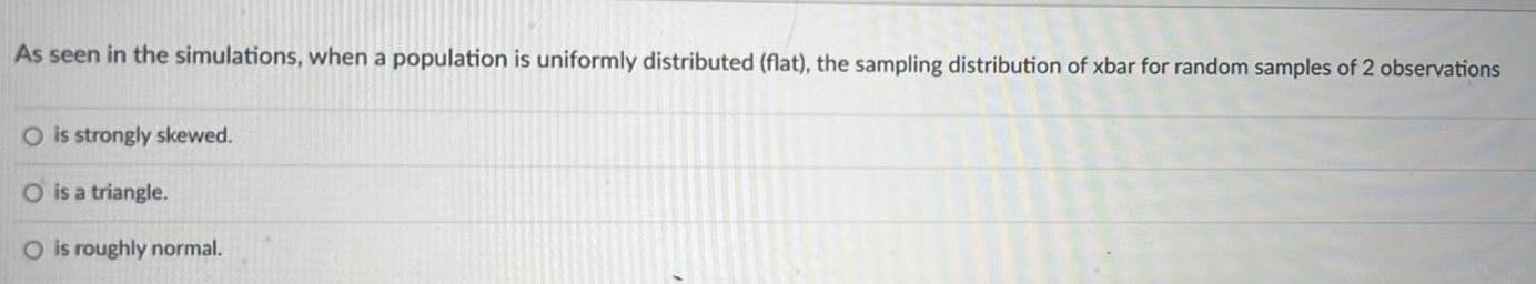
StatisticsAs seen in the simulations when a population is uniformly distributed flat the sampling distribution of xbar for random samples of 2 observations O is strongly skewed O is a triangle O is roughly normal
Statistics
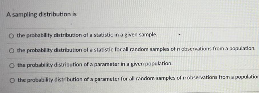
StatisticsA sampling distribution is O the probability distribution of a statistic in a given sample O the probability distribution of a statistic for all random samples of n observations from a population O the probability distribution of a parameter in a given population O the probability distribution of a parameter for all random samples of n observations from a population
Statistics
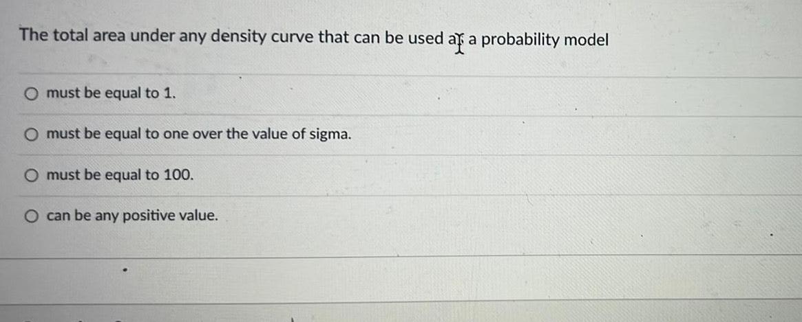
StatisticsThe total area under any density curve that can be used as a probability model O must be equal to 1 O must be equal to one over the value of sigma O must be equal to 100 O can be any positive value
Statistics
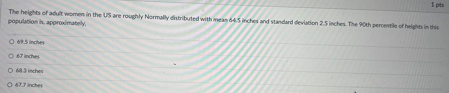
StatisticsThe heights of adult women in the US are roughly Normally distributed with mean 64 5 inches and standard deviation 2 5 inches The 90th percentile of heights in this population is approximately O 69 5 inches O 67 inches O 68 3 inches 1 pts O 67 7 inches
Statistics
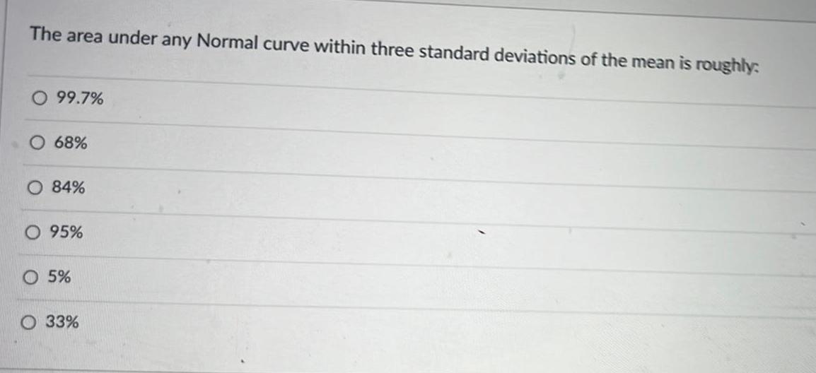
StatisticsThe area under any Normal curve within three standard deviations of the mean is roughly O 99 7 68 84 95 O 5 O 33
Statistics
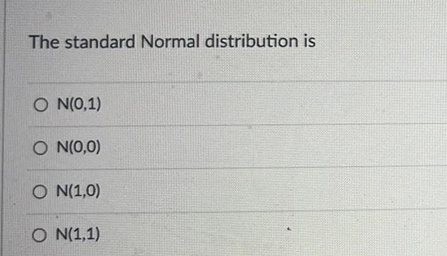
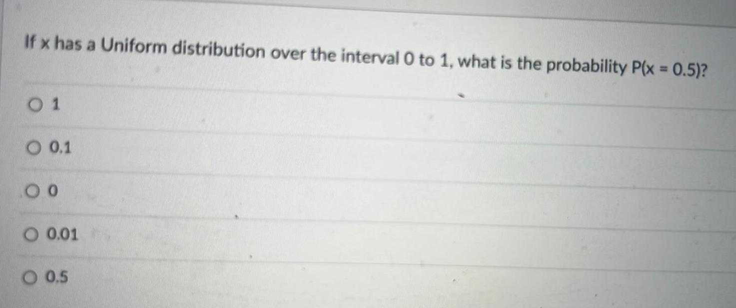
StatisticsIf x has a Uniform distribution over the interval 0 to 1 what is the probability P x 0 5 0 1 O 0 1 00 O 0 01 O 0 5
Statistics
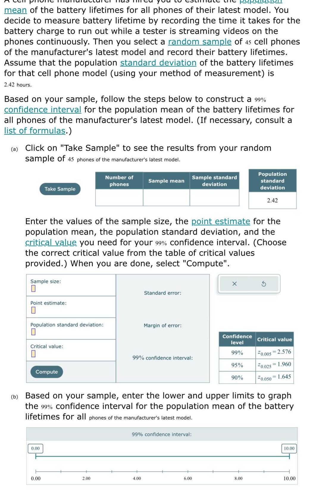
Statisticsmean of the battery lifetimes for all phones of their latest model You decide to measure battery lifetime by recording the time it takes for the battery charge to run out while a tester is streaming videos on the phones continuously Then you select a random sample of 45 cell phones of the manufacturer s latest model and record their battery lifetimes Assume that the population standard deviation of the battery lifetimes for that cell phone model using your method of measurement is 2 42 hours Based on your sample follow the steps below to construct a 99 confidence interval for the population mean of the battery lifetimes for all phones of the manufacturer s latest model If necessary consult a list of formulas a Click on Take Sample to see the results from your random sample of 45 phones of the manufacturer s latest model Take Sample Sample size 0 Point estimate Population standard deviation Critical value Enter the values of the sample size the point estimate for the population mean the population standard deviation and the critical value you need for your 99 confidence interval Choose the correct critical value from the table of critical values provided When you are done select Compute Compute 0 00 0 00 Number of phones 2 00 Sample mean Standard error Margin of error 4 00 99 confidence interval Sample standard deviation 99 confidence interval 6 00 X Confidence level 99 95 b Based on your sample enter the lower and upper limits to graph the 99 confidence interval for the population mean of the battery lifetimes for all phones of the manufacturer s latest model 90 Population standard deviation 2 42 8 00 Critical value 20 005 2 576 20 025 1 960 20 050 1 645 10 00 10 00
Statistics
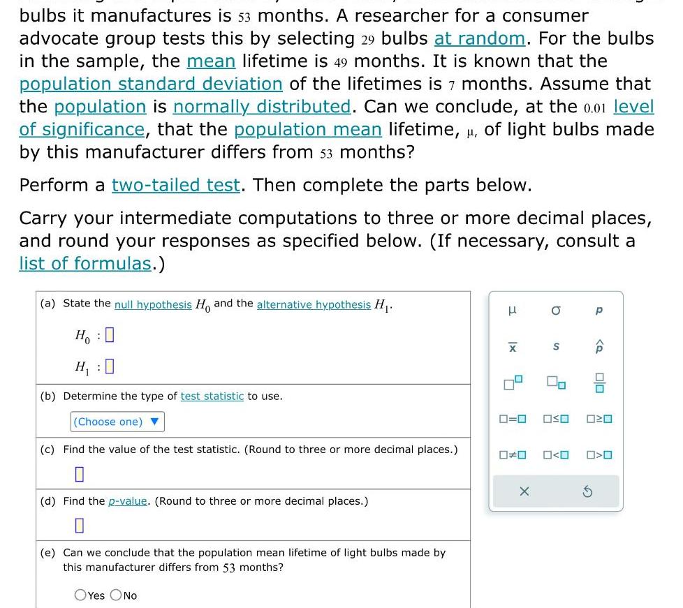
Statisticsbulbs it manufactures is 53 months A researcher for a consumer advocate group tests this by selecting 29 bulbs at random For the bulbs in the sample the mean lifetime is 49 months It is known that the population standard deviation of the lifetimes is 7 months Assume that the population is normally distributed Can we conclude at the 0 01 level of significance that the population mean lifetime of light bulbs made by this manufacturer differs from 53 months Perform a two tailed test Then complete the parts below Carry your intermediate computations to three or more decimal places and round your responses as specified below If necessary consult a list of formulas a State the null hypothesis Ho and the alternative hypothesis H Ho H b Determine the type of test statistic to use Choose one c Find the value of the test statistic Round to three or more decimal places d Find the p value Round to three or more decimal places e Can we conclude that the population mean lifetime of light bulbs made by this manufacturer differs from 53 months OYes ONO X 0 O X S 0 0 OSO 020 0 0 P S P 00 O
Statistics
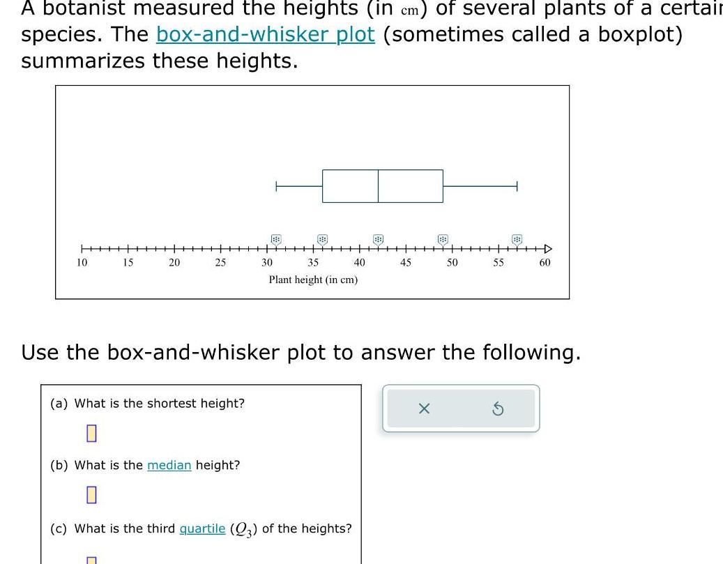
StatisticsA botanist measured the heights in cm of several plants of a certain species The box and whisker plot sometimes called a boxplot summarizes these heights 10 15 20 25 a What is the shortest height n b What is the median height 88 35 30 Plant height in cm 40 c What is the third quartile 23 of the heights 45 Use the box and whisker plot to answer the following 50 X D 55 60
Statistics
StatisticsA town s government is looking into its residents opinion on rebuilding the boardwalk on their coastline Two representatives from the town visit the existing boardwalk and randomly survey 50 people to see whether they support the new boardwalk They find that 62 of those surveyed support the construction of the new boardwalk and conclude that with 90 confidence the majority of residents support its construction What aspect of this scenario brings the validity of this conclusion into doubt 1 point O The 90 confidence interval includes values below 50 O The sample might not be representative of the population of interest O The sample size is not large enough O The conclusion does not report the standard deviation or the confidence interval
Statistics
Probabilitypoint While taking a walk along the road where you live you accidentally drop your glove but you don t know where The probability density p x for having dropped the glove a kilometers from home along the road is p x 4e 4 for x 0 a What is the probability that you dropped it within 1 kilometer of home b At what distance y from home is the probability that you dropped it within y km of home equal to 0 95 km
Statistics
StatisticsWhen is the median the most appropriate measure of central tendency Choose the correct answer below O A When a set of data entries is numerical and there are no entries that are much higher or much lower than the rest O B When a set of data entries is numerical has multiple duplicates and there are no entries that are much higher or lower than the rest OC When a set of data is not numerical O D When the set of data entries is numerical and there is a small number of entries that are much higher or much lower than the rest
Statistics
Statisticstermine whether the following statement is true or false and explain why ample can have more than one mode oose the correct answer below A True a sample can have more than one mode if all values occur once B True a sample can have more than one mode when multiple entries are tied for the largest frequency C False a sample can only have one mode or no mode D False a sample can only have one mode
Statistics
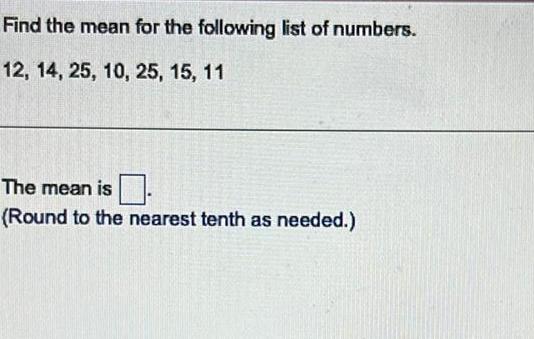
StatisticsFind the mean for the following list of numbers 12 14 25 10 25 15 11 The mean is Round to the nearest tenth as needed
Statistics
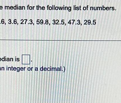
Probabilitye median for the following list of numbers 6 3 6 27 3 59 8 32 5 47 3 29 5 edian is an integer or a decimal

Statistics
StatisticsK Find the percent of the total area under the standard normal curve between the following pair of z 1 1 and z 0 55 Click here to view page 1 of the Areas under the Normal Curve Table Click here to view page 2 of the Areas under the Normal Curve Table In order to find the area between the area under the curve between the two z scores first find the area to the left of each z score The area to the left of z 1 1 is The area to the left of z 0 55 is Round to four decimal places as needed The percent of the total area between z 1 1 and z 0 55 is Round to the nearest whole percent as needed
Statistics
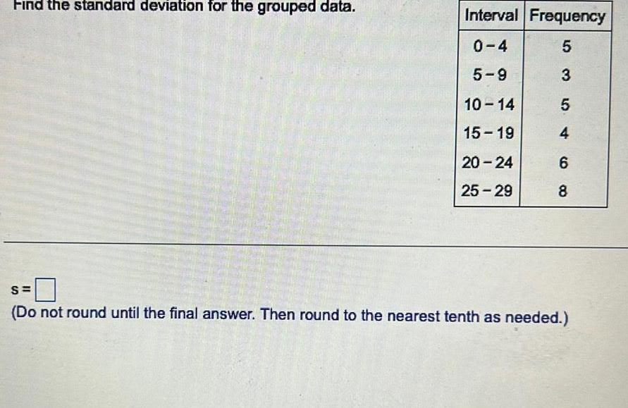
StatisticsFind the standard deviation for the grouped data Interval Frequency 0 4 5 5 9 3 10 14 5 15 19 4 20 24 6 25 29 8 S Do not round until the final answer Then round to the nearest tenth as needed
Statistics
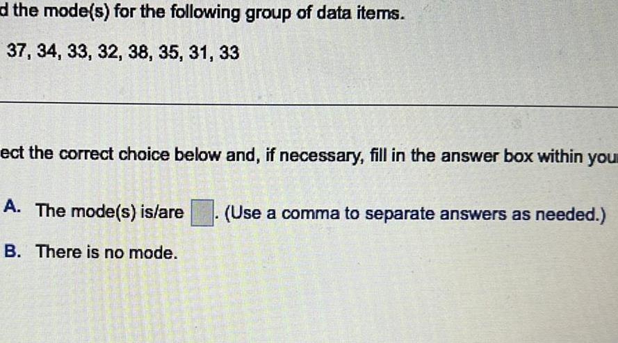
Statisticsd the mode s for the following group of data items 37 34 33 32 38 35 31 33 ect the correct choice below and if necessary fill in the answer box within you A The mode s is are B There is no mode Use a comma to separate answers as needed

Statistics
StatisticsK Use six intervals starting with 0 24 Perform the following a Group the data as indicated b Prepare a frequency distribution with a column for intervals and frequencies c Construct a histogram d Construct a frequency polygon a Tally the given data falling into each interval Choose the correct table below OA OB Interval 0 24 24 48 48 72 H 72 96 96 120 120 149 Tally Will 441 Interval 0 24 25 49 50 74 411 75 99 Hi 100 124 III 125 149 Tally O C Interval 0 24 24 48 48 72 72 96 96 120 120 149 1 Tally 441 1 17 118 115 71 129 25 28 44 127 82 57 136 45 73 63 143 77 72 122 11 46 35 83 82 2 97 84 96 91 36 85 147 32 82 12 101 O D Interval Tally 0 24 Willl LH1 25 49 50 74 75 99 LH1 LH1 IIII 100 124 1 125 149 IIII