Statistics Questions

od restaurant 18 8 31 17 present the number of grams of fat in breakfast meals offere a Construct a stem and leaf plot and b describe the shape of t 18 27 26 10 11 41 13 39 5 18 7 26 6 25 5 31 12 22 Construct the stem and leaf plot below Legend 5 1 represents 51 grams of fat

al survey asked people How often do out for dinner instead of at home The cies were as follows Complete parts a g Response ever arely ometimes ost of the time ways Frequency 332 495 977 509 22 a Construct a relative frequene distribution of the data Response Rela Frequ Never Rarely Sometimes Most of the time Always Round to three decimal places as needed b What percentage of responder answered Always Round to one decimal place

e weight chart shown to e right which is in the agazine style of graph ould the information ovided be organized into Die chart Why or y not Metabolism too slow 59 Don t exercise A No The values in the table are not decimals OB No There are more than 3 categories of data OC Yes The information could be organized into a pie chart OD No The percentages add up to more than 100 50 Don t have self discipline

014 1447 8 35557 9 01 egend 110 represents 10 he original set of data is se a comma to separate answers as needed Use ascend

Medal won in race the variable qualitative or quantitative OA The variable is quantitative because it is an attribute charact OB The variable is quantitative because it is a numerical measur OC The variable is qualitative because it is an attribute character OD The variable is qualitative because it is a numerical measure

The open ended table category class width is the difference between consecutive lower class limits relative frequency frequenou diets

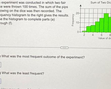
experiment was conducted in which two fair ce were thrown 100 times The sum of the pips owing on the dice was then recorded The quency histogram to the right gives the results se the histogram to complete parts a rough f Frequency 20 10 0 What was the most frequent outcome of the experiment 1 What was the least frequent Sum of Two Dica 6 8 Value of die

What does it mean if a statistic is resistant Choose the correct answer below O A Changing particular data values affects its value substantially OB OC Extreme values very large or small relative to the data affect its value Extreme values very large or small relative to the data do not affect it substantially O D An estimate of its value is extremely close to its actual value

top speed in meters per hour of all the players except tenders in a certain soccer league Find a the aber of classes b the class limits for the third s and c the class width There are e a whole number classes he lower class limit for the third class is an integer or a decimal Do not round upper class limit for the third class is e an integer or a decimal Do not round the class width is Speed km hr Number of Pl 10 13 9 14 17 9 18 21 9 22 25 9 26 29 9 30 33 9 7 17 67 293 177

tion played by the most valuable wer MVP in a certain baseball league the last 84 years Use the chart to wer parts a through d position with the most MVPS was How many MVPs played third base 3B MVPs played third base Frequency 40 35 30 25 20 15 10 5 00 OF 1B 3B PC SS 2B Posit

The rankings of songs in the top 100 Choose the correct level of measurement O Nominal O Ordinal O Interval O Ratio

chart below depicts the beverage size ers choose while at a fast food ant Complete parts a through c opular beverage sizes at a restaurant Small 22 Medium 16 Large 52 XL 10 What percentage of custome this size OA Small 22 OB Large 52 OC Medium 16 O D XL 10 b What is the least popular What percentage of customer this size A Medium 16 OB Large 52 C XL 10 D Small 22

timate the percentage of defects in a recent manufacturing batch a quality conta neral Electric selects every 15th refrigerator that comes off the assembly line sta nth until she obtains a sample of 110 refrigerators type of sampling is used A Cluster 3 Systematic C Convenience D Simple random E Stratified

Goals Is the variable discrete or continuous OA The variable is discrete because it is countable OB The variable is continuous because it is not counta C The variable is discrete because it is not countable D The variable is continuous because it is countable

e whether the underlined value is a parameter or a statistic he interviews of 1 502 adults 18 years of age or older found that only 69 c the current vice president ue a parameter or a statistic The value is a statistic because the 1 502 adults 18 years of age or older are population The value is a statistic because the 1 502 adults 18 years of age or older are The value is a parameter because the 1 502 adults 18 years of age or older a population The value is a parameter because the 1 502 adults 18 years of age or older an sample

Concentration of CO in the Atmosphere Levels of carbon dioxide CO in the atmosphere are rising rapidly far above any levels ever before recorded Levels were around 27 parts per million in 1800 before the Industrial Age and had never in the hundreds of thousands of years before that gone above 300 ppm Levels are now over 400 ppm The table below shows the rapid rise of CO concentrations over the 55 years from 1960 2015 also available in Carbon Dioxide We can use this information to predict CO levels in different years Year 1960 1965 1970 1975 1980 1985 1990 No 1995 2000 2005 2010 2015 The intercept is 2571 Does it make sense in context CO e What is the intercept of the line Round your answer to one decimal place g Find the residual for 2010 316 91 320 04 325 68 331 11 338 75 346 12 354 39 360 82 369 55 379 80 389 90 400 83

Use StatKey or other technology to find the regression line to predict Y from X using the following data Click here to access StatKey X Y Round your answers to two decimal places 10 510 15 469 20 459 25 30 35 460 422 367 40 45 314 252

Levels of carbon dioxide CO in the atmosphere are rising rapidly far above any levels ever before recorded Levels were around 278 parts per million in 1800 before the Industrial Age and had never in the hundreds of thousands of years before that gone above 300 ppm Levels are ny over 400 ppm The table below shows the rapid rise of CO concentrations over the 55 years from 1960 2015 also available in Carbon Dioxide We can use this information to predict CO levels in different years Year 1960 1965 1970 1975 1980 1985 1990 1995 2000 2005 2010 2015 CO 316 91 320 04 Round yo 325 68 331 11 338 75 346 12 354 39 360 82 369 55 379 80 389 90 400 83 a What is the explanatory variable What is the response variable O CO concentration is the explanatory variable and Year is the response variable Year is the explanatory variable and CO concentration is the response variable b Use technology to find the correlation between year and CO2 level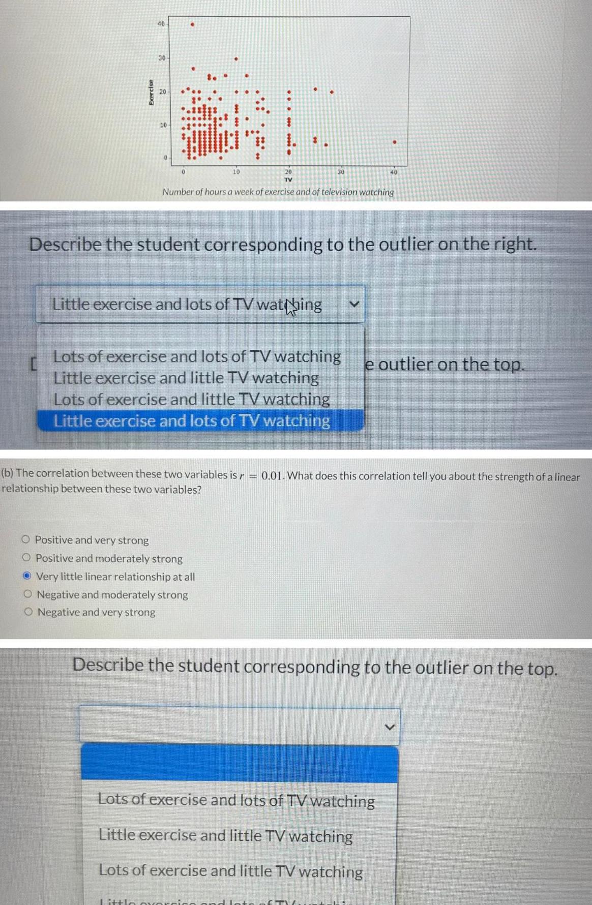s

The StudentSurvey dataset includes information on the number of hours a week students say they exercise and the number of hours a week students say they watch television D 40 C 20 10 Click here for the dataset associated with this question a There are two outliers in this scatterplot 20 TV Number of hours a week of exercise and of television watching Describe the student corresponding to the outlier on the right Little exercise and lots of TV watching O Positive and very strong 30 e outlier on the top Lots of exercise and lots of TV watching Little exercise and little TV watching Lots of exercise and little TV watching Little exercise and lots of TV watching Describe the student corresponding to the outlier on the top Lots of exercise and lots of TV watching Little exercise and little TV watching Lots of exercise and little TV watching Little exercise and lots of TV watching b The correlation between these two variables is r 1 0 01 What does this c b The correlation between these two variables is r 0 01 What does this correlation tell you about the strength of a linea relationship between these two variables

Exercise 40 30 20 10 0 10 20 TV Number of hours a week of exercise and of television watching Little exercise and lots of TV watching Describe the student corresponding to the outlier on the right O Positive and very strong O Positive and moderately strong Lots of exercise and lots of TV watching Little exercise and little TV watching Lots of exercise and little TV watching Little exercise and lots of TV watching Very little linear relationship at all O Negative and moderately strong O Negative and very strong 30 Little overe b The correlation between these two variables is r 0 01 What does this correlation tell you about the strength of a linear relationship between these two variables 40 V STV e outlier on the top Describe the student corresponding to the outlier on the top Lots of exercise and lots of TV watching Little exercise and little TV watching Lots of exercise and little TV watching

new attraction a survey was done at this year s state fair It was found that among a random sample of 65 couples at the fair with their children 43 had visited the new miniature golf course and among an independently chosen random sample of 73 couples at the fair on a date without children 49 had visited the miniature golf course Based on these samples can we conclude at the 0 10 level of significance that the proportion p of all couples attending the fair with their children who visited the miniature golf course is different from the proportion p of all couples attending the fair on a date who visited the miniature golf course Perform a two tailed test Then complete the parts below Carry your intermediate computations to three or more decimal places and round your answers as specified in the parts below If necessary consult a list of formulas a State the null hypothesis H and the alternative hypothesis H Ho 0 H 0 b Determine the type of test statistic to use Choose one c Find the value of the test statistic Round to three or more decimal places 0 d Find the p value Round to three or more decimal places 0 e Can we conclude that the proportion of couples visiting the miniature golf course is different between the two populations 3 X 0 O X a S OSO O O P D 00 O

TV Hours Over a Decade The PASeniors dataset has survey data from a sample of Pennsylvania high school seniors who participated in the Census at Schools project over the decade from 2010 to 2020 One of the variables TVHours asks about number of hours spent watching TV each week To see how that variable might change over the decade we run a regression where the explanatory variable t measures time in years over the decade with t 0 in 2010 and t 10 in 2020 The fitted line predicting the average weekly hours of TV each year is TVHours 8 835 0 397t Based on the fitted line about how much has the average weekly TV hours increased or decreased over this decade hours per week by i

Which plot below would correlation not be an accurate summary of the association O Land vs Water 35 0 4 30 0 3 0 2 Car Weight vs Overall MPG 404 0 14 15 25 20 2000 404 304 0 6 20 O Land Size vs Population Size 10 3000 Rent vs Price 0 7 C00 I 4000 0 8 000 5000 0 9 40 6000 andraba 50

The box plot and 5 number summary below displays the percentage of Southwest airline flights that departed on time per day for 200 days in 2018 0 4 0 2 0 0 0 2 0 41 50 Min Q1 Median Mean Q3 Max 44 63 66 66 5 70 85 60 On time Percentage 70 For each statement below answer T if the statement is true and F is the statement is false Bold for emphasis you don t need to enter a bold letter just T or F The percentage of on time departures is right skewed A majority of the days have fewer than 66 5 of flights depart on time The percentage of on time departures is right skewed There are the same number of days in the sample with an on time departure percentage above 70 as days below 63 80 There are no days with an unusually low or high percent of flights that departed on time About 50 days in the cample had 70 or more flights donarton

QUESTION 5 Which plot below would correlation be an accurate summary of the association Car Type vs Car Weight Weight 4000 3500 3000 2500 2000 O Car Weight vs Overall MPG 40 35 30 25 20 15 300 250 40 200 Car Weight vs Displacement Displacement 350 150 2000 100 504 10 50 Small 304 204 Land Size vs Population Size U 2000 3000 Compact BOS B 5000 10 2500 80 4000 Type one come so N MOD 3000 Weight 5000 Medium 3500 6000 4000 Large

O Scatterplot 1 50 40 30 20 O Scatterplot 2 10 50 40 30 20 10 0 41 0 31 40 0 2 35 0 1 Scatterplot 4 Scatterplot 3 60 304 55 254 50 45 40 35 0 6 304 Scatterplot 5 10 10000000 0 7 20000000 com 00 0 8 40 30000000 45 0 9 40 50

A study was conducted to determine if there was a difference in the amount of television watched in a week recorded in hours between men and women The data was collected and summarized as you see below Dotplot Histogram Box plot F M 0 5 10 15 I 20 25 30 35 40 Identify the explanatory and response variables for this study and discuss the relationship between the two variables Summary Statistics Statistics Sample Size Mean Standard Deviation Minimum Q Median Q3 Maximum M 192 7 620 6 427 0 3 00 5 00 10 00 40 F 169 5 237 4 100 0 3 00 4 00 6 00 20 Overall 361 6 504 5 584 0 3 00 5 00 9 00 40

Emma s On the Go a large convenience store that makes a good deal of money from candy bar sales has three possible locations in the store for its candy bar display in the front of the store to attract impulse buying by all customers on the left hand side of the store to attract teenagers who are on that side of the store looking at the soda and in the back of the store to attract the adults searching through the alcohol cases The manager at Emma s experiments over the course of many months by rotating the candy bar display among the three locations choosing a sample of 43 days at each location Each day the manager records the amount of money brought in from the sale of candy bars Below are the sample mean daily sales in dollars for each of the locations as well as the sample variances Group Front of store Left hand side Back of store Sample Sample Sample size mean variance 43 226 9 551 8 43 221 1 276 4 43 218 9 506 0 Send data to calculator V Send data to Excel Suppose that we were to perform a one way independent samples ANOVA test to decide if there is a significant difference in the mean daily sales among the three locations Answer the following carrying your intermediate computations to at least three decimal places and rounding your responses to at least one decimal place a What is the value of the between groups mean square that would be reported in the ANOVA test b What is the value of the within groups mean square that would be reported in the ANOVA test

Among the huge body of literature on smoking are data detailing the relative successfulness of males and females in quitting smoking A study of 400 adults who began various smoking cessation programs produced the data in the contingency table below The table shows data from the study regarding two variables the smoker s sex male or female and the length of the smoking cessation period less than two weeks between two weeks and one year or at least one year In the table less than two weeks means that the individual returned to smoking within two weeks of beginning the program between two weeks and one year means that the individual survived the first two weeks but returned to smoking within a year and at least one year means that the individual did not smoke for at least a year after beginning the program The cells of the table each contain three numbers The first number in each cell is the observed cell frequency o the second number is the expected cell frequency under the assumption that there is no association between sex and the length of the smoking cessation period and the third number is the following value fo E Observed cell frequency Expected cell frequency Expected cell frequency The numbers labeled Total are totals for observed frequency Part 1 Fill in the missing values in the contingency table Round your expected frequencies to two or more decimal places and round your values to three or more decimal places Send data to Excel Sex Male Female Total 0 Length of smoking cessation period Less than two weeks 69 0 0 34 0 0 103 a Determine the type of test statistic to use Type of test statistic Choose one Yes No Yes Between two weeks At least one and one year year 136 128 63 0 422 74 81 38 0 669 210 40 0 0 47 0 0 87 Total 245 155 400 Part 2 Answer the following to summarize the test of the hypothesis that there is no association between sex and the length of the smoking cessation period For your test use the 0 10 level of significance b Find the value of the test statistic Round to two or more decimal places c Find the critical value for a test at the 0 10 level of significance Round to two or more decimal places d Can we conclude that there is an association between sex and the length of the smoking cessation period Use the 0 10 level of significance fo fE JE X X 5

procedures Option 1 and Option 2 to load passengers onto their Long Beach LGB to San Francisco SFO flights Since Option 1 has more automation the airline suspects that the mean Option 1 loading time is less than the mean Option 2 loading time see if this is true the airline selects a random sample of 275 flights from LGB to SFO using Option 1 and records their loading times The sample mean is found to be 17 8 minutes with a sample standard deviation of 5 3 minutes They also select an independent random sample of 220 flights from LGB to SFO using Option 2 and record their loading times The sample mean is found to be 18 2 minutes with a sample standard deviation of 4 2 minutes Since the sample sizes are quite large it is assumed that the population standard deviation of the loading times using Option 1 and t loading times using Option 2 can be estimated to be the sample standard deviation values given above At the 0 10 level of significance is there sufficient evidence to support the claim that the mean Option 1 loading time is less than the mean Option 2 loading time for the airline s flights from LGB to SFO Perform a one tailed test Then complete the parts below Carry your intermediate computations to at least three decimal places If necessary consult a list of formulas a State the null hypothesis Ho and the alternative hypothesis H Ho H 0 b Determine the type of test statistic to use Choose one c Find the value of the test statistic Round to three or more decimal places 0 d Find the p value Round to three or more decimal places 0 e Can we support the claim that the mean Option 1 loading time is less than the mean Option 2 loading time for the airline s flights from LGB to SFO OXES ONO F X 0 0 O X S OSO O 0 0 P Q P olo 20 O

A worldwide organization of academics claims that the mean IQ score of its members is 112 with a standard deviation of 16 A randomly selected group of 35 members of this organization is tested and the results reveal that the mean IQ score in this sample is 114 6 If the organization s claim is correct what is the probability of having a sample mean of 114 6 or less for a random sample of this size Carry your intermediate computations to at least four decimal places Round your answer to at least three decimal places

For each of the variables described below indicate whether it is a quantitative or a categorical qualitative variable Al ndicate the level of measurement for the variable nominal ordinal interval or ratio Make sure your responses are th most specific possible Variable a Temperature in degrees Celsius b Amount in pounds of weight needed to break a bridge cable c Name of manufacturer of an automobile Type of variable OQuantitative Categorical OQuantitative Categorical OQuantitative OCategorical Level of measurement Nominal OOrdinal Interval O Ratio ONominal Ordinal Interval Ratio Nominal Ordinal O Interval O Ratio X

The 10 members of the swim team completed the following numbers of laps at today s practice 22 78 79 81 85 88 89 91 91 154 Complete the parts below to identify any outliers a Let o be the lower quartile and o3 be the upper quartile of the data set Find 2 and 23 for the data set Q 0 9 0 b Find the interquartile range IQR of the data set IQR Lower boundary Upper boundary X c Calculate a lower boundary using Q 1 5 IQR Calculate an upper boundary using Q3 1 5 IQR Note that 1 5 IQR means 1 5 times the IQR Outliers X S d Any values less than the lower boundary or greater than the upper boundary are considered outliers Identify all the outliers of the data set If there is more than one outlier separate them with commas If there are no outliers click None None

a A manager at a bus company wants to survey employees about the new uniforms Which of the following best describes a systematic sample of employees The manager uses a computer program to draw 72 employees at random and selects these employees Every set of 72 employees is equally likely to be drawn by the computer program The manager forms 6 groups of employees based on the departments the employees are in Then she selects 12 employees at random from each group The manager takes a list of the employees and selects every 3rd employee until 72 employees are selected b A facilities supervisor at a sports stadium wants to rate the condition of the seats at the stadium Which of the following best describes a convenience sample of seats The supervisor uses a computer program to draw so seats at random and selects these seats Every set of so seats is equally likely to be drawn by the computer program The supervisor takes a list of the seats and selects every 5th seat until 50 seats are selected All of the seats in the VIP section are easily accessible So the supervisor selects the so seats in this section c A consultant wants to ask workers at a factory about the workers job satisfaction Which of the following best describes a stratified sample of workers The consultant forms groups of 30 workers based on the lengths of time the workers have worked at the factory Then he randomly chooses 3 groups and selects all of the workers in these groups The consultant forms 5 groups of workers based on the workers shifts Then he selects 18 workers at random from each group All of the workers on the second floor of the factory building are easily accessible So the consultant selects the first 90 workers from the second floor to arrive at work on a particular day

Here are the shopping times in minutes for a sample of 6 shoppers at a particular grocery store 42 43 40 44 35 24 Send data to calculator Find the standard deviation of this sample of shopping times Round your answer to two decimal places If necessary consult a list of formulas

The ages in years of the 5 doctors at a local clinic are the following 44 53 41 40 37 Send data to calculator Send data to Excel Assuming that these ages constitute an entire population find the standard deviation of the population Round your answer to two decimal places If necessary consult a list of formulas

The following list contains the number of hours that a sample of 11 middle school students spent watching television last week 4 7 18 9 18 12 13 7 8 13 17 Send data to calculator Send data to Excel Find the median number of hours for that sample hours 5

In an experimental study researchers had each of the participants bet on each game of a professional football season The contingency table below contains some information from a random sample of 100 bets placed on the Columbus Crush picking them to win during the last 14 games of the season the Crush had 7 wins and 7 losses over that period This contingency table indicates for each bet placed on the Crush whether or not the team won and how the participant who placed the bet went the following week So there are two variables represented result of picking the Crush Crush won or Crush lost and bet placed the following week picked Crush to win or picked Crush to lose Each cell of the table contains three numbers the first number is the observed cell frequency the second number is the expected cell frequency f under the assumption that there is no dependence between the two variables result of picking the Crush and bet placed the following week and the third number is the following value fo fe Observed cell frequency Expected cell frequency Expected cell frequency The numbers labeled Total are totals for observed frequency Part 1 Fill in the missing values in the contingency table Round your expected frequencies to two or more decimal places and round your values to three or more decimal places SE Send data to Excel Result of picking the Crush Crush won Crush lost Total 0 Bet placed the following week Picked Crush Picked Crush to win to lose 33 0 0 35 0 0 68 a Determine the type of test statistic to use Type of test statistic Choose one Yes Yes No 22 0 0 10 0 0 32 Total 55 Part 2 Answer the following to summarize the test of the hypothesis that there is no dependence between the two variables result of picking the Crush and bet placed the following week For your test use the 0 10 level of significance 45 100 b Find the value of the test statistic Round to two or more decimal places 0 c Find the critical value for a test at the 0 10 level of significance Round to two or more decimal places d Can we reject the hypothesis that there is no dependence between the variables result of picking the Crush and bet placed the following week Use the 0 10 level of significance S

togram of a sample from a population with a skewed distribution one is the distribution of many means of repeated random samples of size 5 and one is the distribution of repeated means of random samples of size 25 all the samples are from the same population State which is which and how you know A B C

on each game of a professional football season The contingency table below contains some information from a random sample of 100 bets placed on the Columbus Crush picking them to win during the last 14 games of the season the Crush had 7 wins and 7 losses over that period This contingency table indicates for each bet placed on the Crush whether or not the team won and how the participant who placed the bet went the following week So there are two variables represented result of picking the Crush Crush won or Crush lost and bet placed the following week picked Crush to win or picked Crush to lose Each cell of the table contains three numbers the first number is the observed cell frequency the second number is the expected cell frequency f under the assumption that there is no dependence between the two variables result of picking the Crush and bet placed the following week and the third number is the following value fo fE Observed cell frequency Expected cell frequency Expected cell frequency The numbers labeled Total are totals for observed frequency Part 1 Fill in the missing values in the contingency table Round your expected frequencies to two or more decimal places and round your values to three or more decimal places JE Send data to Excel Result of picking the Crush Crush won Crush lost Total Bet placed the following week Picked Crush Picked Crush to win to lose 12 0 0 18 0 0 30 45 10 0 25 0 0 70 a Determine the type of test statistic to use Type of test statistic Choose one Total Yes No 57 43 100 Part 2 Answer the following to summarize the test of the hypothesis that there is no dependence between the two variables result of picking the Crush and bet placed the following week For your test use the 0 10 level of significance b Find the value of the test statistic Round to two or more decimal places 0 c Find the p value Round to three or more decimal places 0 d Can we reject the hypothesis that there is no dependence between the variables result of picking the Crush and bet placed the following week Use the 0 10 level of significance X S X

9 36 Tomatoes The weights of four randomly and independently elected bags of tomatoes labeled 5 pounds were found to be 5 1 5 0 5 3 and 5 1 pounds Assume Normality a Find a 95 confidence interval for the mean weight of all bags of tomatoes b Does the interval capture 5 0 pounds Is there enough evidence to reject a mean weight of 5 0 pounds

TRY 9 15 CLT Shapes Example 4 One of the histograms is a his togram of a sample from a population with a skewed distribution one is the distribution of many means of repeated random samples of size 5 and one is the distribution of repeated means of random samples of size 25 all the samples are from the same population State which is which and how you know A B C

18 Student Ages The mean age of all 2550 students at a small ollege is 22 8 years with a standard deviation is 3 2 years and the istribution is right skewed A random sample of 4 students ages is btained and the mean is 23 2 with a standard deviation of 2 4 years a o x s b Is a parameter or a statistic c Are the conditions for using the CLT fulfilled What would be the shape of the approximate sampling distribution of many means each from a sample of 4 students Would the shape be right skewed Normal or left skewed

9 2 Units A survey of 100 random full time students at a large university showed the mean number of semester units that students were enrolled in was 15 2 with a standard deviation of 1 5 units a Are these numbers statistics or parameters Explain b Label both numbers with their appropriate symbol such as x u s or

9 17 Used Car Ages Example 5 The mean age of all 638 used cars for sale in the Ventura Country Star one Saturday in 2013 was 7 9 years with a standard deviation of 7 7 years The distribu ion of ages is right skewed For a study to determine the reliability of classified ads a reporter randomly selects 40 of these used cars and plans to visit each owner to inspect the cars He finds that the mean age of the 40 cars he samples is 8 2 years and the standard Heviation of those 40 cars is 6 0 years a Which of these four numerical values are parameters and which are statistics b s x c Are the conditions for using the CLT fulfilled What would be the shape of the approximate sampling distribution of a large number of means each from a sample of 40 cars

9 1 Ages A study of all the students at a small college showed a mean age of 20 7 and a standard deviation of 2 5 years a Are these numbers statistics or parameters Explain b Label both numbers with their appropriate symbol such as x u s or o

9 23 College Admission Rates Example 7 A random sample of 10 colleges from Kiplinger s 100 Best Values in Public Education was taken A 95 confidence interval for the mean admission rate was 52 8 75 0 The rates of admission were Normally distrib ted Which of the following statements is a correct interpretation of the confidence level and which is the correct interpretation of he confidence interval Source http portal kiplinger com tool college T014 S001 kiplinger s best values in public colleges index php colleges Accessed via StatCrunch Owner Webster West a We are confident that the mean admission rate is between 52 8 and 75 0 b In about 95 of all samples of 10 colleges the confidence interval will contain the population mean admission rate

ry It was a common practice in Southern California for houses to be built with pools in the backyard For new homes howeve that practice may be changing possibly as a measure to help reduce climate change A recent study examined a random sample of 166 houses built in Southern California in the twentieth century and an independent random sample of 74 new houses built in Southern California The sample of twentieth century houses contained 86 houses with pools and the sample of new houses contained 34 houses with pools Based on this survey can we conclude at the 0 01 level of significance that the proportion p of all Southern California twentieth century houses the were built with pools is greater than the proportion p2 of all new Southern California houses that were built with pools Perform a one tailed test Then complete the parts below Carry your intermediate computations to three or more decimal places and round your answers as specified in the parts below If necessary consul a list of formulas a State the null hypothesis Ho and the alternative hypothesis H H 0 H 0 b Determine the type of test statistic to use Choose one c Find the value of the test statistic Round to three or more decimal places 0 d Find the p value Round to three or more decimal places 0 e Can we conclude that the proportion of Southern California twentieth century houses built with pools is greater than the proportion for new homes OX ONO I x X 5 O 0 0 OSO X S P Q olo 20 0 0 0

4 Write five numbers such that the mean is 2 and the variance is zero Opcwort

8 The adult population on a cruise ship has a total of 1564 and can be divided into 3 educational level categories B adults with less than high school B adults with high school diploma and B3 adults with a baccalaureate or more The probabilities of selecting an adult at random within these categories are P B 7 4 P B 53 3 and P B3 39 3 Certain percent of the adults in each educational level category read an astrology report every day event A The percentages are P A B 9 P A B 7 and P A B3 4 For one of these adults selected at random determine the probability that he or she a reads an astrology report every day Answer P A b is an adult with a high school diploma given that he or she reads an astrology report every day Answer P B 4