Statistics Questions

24 When constructing a pie chart the numbers 100 and 360 are used Describe each number in this context and explain the reason each is necessary

Eight athletes reported their height in meters and their time on the 100 yard dash in seconds as found in the table below a a Plot the data using technology then choose the best description below O positive linear correlation negative linear correlation Slope m Height y Time 9 9 1 6 1 65 10 05 1 6 10 5 1 6 10 4 1 95 10 05 2 10 05 2 10 4 1 95 10 4 no linear correlation b No matter what you said above find the slope and y intercept of the regression line Round answers to three decimal places

A room contains 26 people who would respond differently to a yes no question if asked Room 26 total people 14 people would say Yes 12 people would say No You randomly sample 8 people from the room and record each person s response yes or no Sampling is done WITHOUT replacement Compute the probability of the following events You can enter each solution as a mathematical expression or a number in decimal form with 5 decimal places included YYNYYYNN a b YNYNNYYY

Submit quiz A town s January high temperatures average 37 F with a standard deviation of 10 while in July the mean high temperature is 77 and the standard deviation is 6 In which month is it more unusual to have a day with a high temperature of 55 Explain Select the correct choice below and fill in the answer boxes within your choice Round to three decimal places as needed A It is more unusual to have a day with a high temperature of 55 in July A high temperature of 55 in July is standard deviations below the mean and a high temperature of 55 in January is only standard deviations above the mean OB It is more unusual to have a day with a high temperature of 55 in January A high temperature of 55 in January is standard deviations above the mean and a high temperature of 55 in July is only standard deviations below the mean

PART III Statistical Concepts Applied Questions Complete each of the following problems Show enough on your paper for me to see what you are thinkin as you work through the exercise Write in complete sentences whenever you are asked WHY or to EXPLAIN your answer 17 The time required for 10 children to learn a particular motor skill was recorded as 9 15 23 20 16 15 24 18 10 and 20 minutes a Find the mean and the median time to learn this task use appropriate labels for the data b Based on the values of the mean and median are the measurements symmetric or skewed WHY

9 A sample of 600 values produced the following summary descriptive statistics upper Q1 35 6 Q2 54 2 Q3 62 4 Mean 56 8 Given this information the fence on a box whisker plot is b 4 60 a 26 80 d 102 60 c 75 80 10 Given a distribution of measurements that is approximately mound shaped the Empirical Rule states that the approximate percentage of measurements in a data set that fall within 1 standard deviation of their mean is approximately a 99 b 95 c 90 d 68 true or F for false

When a data set is bimodal that means it has a No symmetry b A small range value Which of the following LEAST belongs with the other 3 with respect to the level of measurement scaling a Yearly income in dollars c Capacity of containers in liters b Height in cm d Rank order of the top 5 finalist at MathCounts c Two modes d A large mean value

18 Identify the following variables as either Quantitative QN or Qualitative QL a The brands of ice cream that you might purchase b The daily high temperature for the last 4 weeks c The amount of sugar consumed by Americans each year d The species of fish in Golden Lake e The lengths of time children wait for the school bus f Your favorite NFL team such as the Las Vegas Raiders 19 A math teacher would like to present the midterm results to his class in a way that shows the overall spread of the data The 25 test scores for the math midterm are listed below Construct a graph of your choice use an appropriate heading for the graph and interpret the data set 62 50 98 89 57 79 80 68 65 78 45 78 73 70 73 91 61 72 62 64 50 77 69 82 95

PART II True or False Circle T for true or F for false 11 T or F In the term frequency distribution frequency refers to the number of data values or measurements falling within each class 12 T or F A discrete quantitative variable is one that can assume values only at specific points on an interval of values with inevitable gaps between them 13 T or F A continuous quantitative variable is one that can assume values at all points on an interval of values with no gaps between possible values 14 T or F When a distribution has more values to the left and tails to the right we say it is left skewed 15 T or F To have valid results you must survey everyone in the population of interest 16 T or F In a line chart the horizontal axis represents time such as months years and the vertical axis represents the value of the variable of interest PART III Statistical Concepts Applied Questions Complete each of the following problems Show enough on your paper for me to see what you are thinking Write in complete sentences whenever you are asked WHY or to

be If the manager of a grocery store wishes to display the sales trend the most effective type of graph wil a A bar chart b A pie chart The range of a set of data is a measure of the a Center b Variability c A histogram d A line chart c Middle value d Population

Which of the following statements about mean is NOT always correct a The sum of the deviations from the mean is zero b Half of the observations are on either side of the mean c The mean is a measure of the middle center of a distribution d The value of the mean times the number of observations equals the sum of all of the observations 78 2 a mode 67 and a median 67 A sample of students who has taken a calculus test has a mean Based on this information the distribution of scores is c left skewed b right skewed a symmetric d bimodal The average score for a class of 35 students was 70 The 20 male students in the class averaged 73 The 15 female students in the class averaged a 73 b 70 c 66 d 60

Choose the BES ARTI Multiple Choice A politician who is running for the office of governor of a state with 7 million registered voters commissions a survey In the survey 55 of the 10 000 registered voters interviewed say they plan to vote for her The population of interest is the a 7 million registered voters in the state b 10 000 registered voters interviewed c 55 or 5 500 voters interviewed who plan to vote for her d 45 or 4 500 voters interviewed who plan not to vote for her nd the most effective type of graph will

erentiate H u u V V Set eed Help mit Answer 2 Points rentiate 7 3x 4 3 Read It DETAILS PREVIOUS A

Environmental Protection Agency EPA fuel economy estimates for automobile models tested recently predicted a mean of 24 76 mpg and a standard deviation of 6 17 mpg for highway driving Assume that a Normal model can be applied Use the 68 95 99 7 Rule to complete parts a through e 68 95 99 7 625 1242 18 50 24 76 30 93 37 10 4327 Q B SOCCORS c About what percent of autos should get more than 30 93 mpg Using the 68 95 99 7 Rule about of autos should get more than 30 93 mpg Type an integer or a decimal Do not round d About what percent of autos should get between 30 93 and 37 10 mpg Using the 68 95 99 7 Rule about of autos should get between 30 93 and 37 10 mpg Type an integer or a decimal Do not round e Describe the gas mileage of the worst 2 5 of cars The worst 2 5 of cars get than mpg b In what interval would you expect the central 99 7 of autos to be found Using the 68 95 99 7 Rule the central 99 7 of autos can be expected to be found in the interval from to mpg Type integers or decimals Do not round Use ascending order A 68 95 99 7 625 934 1551 24 76 34 02 40 19 43 27 Q G A

A forester measured 23 of the trees in a large woods that is up for sale He found a mean diameter of 10 9 inches and a standard deviation of 4 2 inches Suppose that these trees provide an accurate description of the whole forest and that a Normal model applies a Choose the correct Normal model for tree diameters OA M 20 pre Ap 20 17 25 67 109 15 1 103 215 a Be 1 20 36 a G b What size would you expect the central 95 of all tree diameters to be Using the 68 95 99 7 rule the central 95 of the tree diameters are between inches and inches Do not round Type integers or decimals O C 109151 193 as 27

Activity A B C D E F G H 1 Predecessor s A A A B C D E E F G H Figure 7 6 Network Scheduling Data Duration days 5 20 15 in 5 60 050 15 20 15 2 Consider the network scheduling data presented in Figure 7 6 How many days of slack are associated with activity E a 0 b 107

Macmillan Learning Enzymatic activity is known to be affected by temperature A study examined the activity rate in micromoles per second mol s of the digestive enzyme acid phosphatase in vitro at varying temperatures measured in kelvins K The findings are displayed in the following table For reference the range of 253 to 298 K corresponds to roughly 25 to 80 degrees Celsius or 77 to 176 degrees Fahrenheit Temperature K 298 298 298 303 303 303 308 308 308 313 313 313 Rate u mol s 0 04 0 05 0 05 0 08 0 08 0 08 0 11 0 13 0 11 0 18 0 20 0 19 Temperature K 318 318 318 323 323 323 323 328 328 333 333 333 Rate mol s 0 34 0 34 0 35 0 47 0 48 0 48 0 48 0 78 0 79 0 97 0 98 1 03 Temperature K 338 338 338 343 343 343 348 348 348 353 353 353 To access the complete data set click the link for your preferred software format Excel Minitab14 18 Minitab 18 JMP SPSS TI R Mac TXT PC TXT CSV CrunchIt Rate mol s 1 05 1 10 1 06 0 96 0 98 0 99 0 72 0 73 0 75 0 54 0 58 0 62 Use the software of your choice to make a scatterplot If you calculate the correlation based on the data provided you find r 0 81 check for yourself 1 M E Petersone et al The dependence of enzyme activity on temperature determination and validation of parameters Biochemical Journal 402 2007 pp 331 337 doi 10 1042 BJ20061143 Explain why the numerical value of the correlation is only moderately strong even though the scatterplot indicates that the effect of temperature on enzymatic activity is clear and very reliable As the value of r is more sensitive to scatter when the relationship is curved the moderate strength of the value of r is due to the scatter of points for higher temperature values The value of r does not have meaning because the relationship is clearly not linear The association is neither positive nor negative The moderate strength of the positive value of r is a consequence of the change in relationship direction from positive to negative with the higher temperature values Although the relationship between the variables is positive for most values the moderately strong positive value of r

The roundworm Caenorhabditis elegans is a widely studied animal model in part because of its small number of neurons and easily manipulated genome Nociception is the neural perception of an actually or potentially harmful stimulus In C elegans it evokes a self preserving withdrawal behavior However repeated stimulation can result in reduced withdrawal response or habituation Researchers compared the withdrawal response to disturbing light stimuli in wild type C elegans and a mutant C elegans line that exhibits a slower response of sensory neurons PVD The given scatterplot shows the data of the percent of animals tested that exhibited a withdrawal reaction to a noxious stimulus consisting of varying numbers of consecutive light pulses Failure to react indicates habituation Circles represent wild type C elegans and squares represent the mutant line Percent of animals reacting 100 60 40 20 Wild type Mutant 10 15 Number of light pulses 20 1 S J Husson et al Optogenetic analysis of a nociceptor neutron and network reveals ion channels acting downstream of primary sensors Current Biology 22 2012 pp 743 753 doi 10 1016 j cub 2012 02 066 Macmillan Learning What does the scatterplot show about the pattern of withdrawal responses in wild type C elegans for increasing numbers of light pulses How does your answer fit in the context of habituation What does the scatterplot show about the pattern of withdrawal responses in wild type C elegans for increasing numbers of light pulses How does your answer fit in the context of habituation O The negative linear association in the wild type C elegans does not indicate habituation The response to the harmful stimulus is more pronounced when the stimulus is applied more times The negative linear association in the wild type C elegans does not indicate habituation The response to the harmful stimulus is less pronounced when the stimulus is applied more times O The negative linear association in the wild type C elegans indicates habituation The response to the harmful stimulus is more pronounced when the stimulus is applied more times The negative linear association in the wild type C elegans indicates habituation The response to the harmful stimulus is less pronounced when the stimulus is applied more times

John Beale of Stanford California recorded the speeds of cars driving past his house where the speed limit read 30 mph The mean of 100 representative readings was 33 63 mph with a standard deviation of 3 44 mph a How many standard deviations from the mean would a car going the speed limit be b Which would be more unusual a car traveling 43 mph or one going 21 mph a A car traveling at the speed limit is 1 06 standard deviations from the mean Round to two decimal places as needed O b Choose the correct answer below and fill in the answer box es to complete your choice Round to two decimal places as needed OA The car traveling 21 mph is more unusual It is B The car traveling 43 mph is more unusual It is Oc Both cars are equally unusual Both cars are standard deviations from the mean while the car traveling 43 mph is standard deviations from the mean while the car traveling 21 mph is standard deviations from the mean standard deviations from the mean standard deviations from the mean

The average score on the Stats midterm was 73 points with a standard deviation of 6 points and Karl s z score was 2 How many points did he score nginte

ne season baseball player A hit 61 home runs During a different season baseball player B hit 54 home runs How does the performance of player A compare to the performance of player B T ble available below shows the means and standard deviations for the number of home runs scored by all players with at least 502 plate appearances in their respective seasons Use these to etermine whose home run feat was more impressive i Click the icon to view the means and standard deviations for the two seasons The z score for player A z is Round to two decimal p than the z score for player B Z Mean Standard deviation CUP so the feat by player Season with Player A 19 3 13 07 Means and Standard Deviations for the Two Seasons was more impressive X Season with Player B 21 3 12 45

Mary s score on the Stats midterm was 69 points The class average was 81 and the standard deviation was 6 points What was her z score z 0

y Side College freshmen involved in a dating relationship agreed to participate in a nine month long study Every two weeks participants answered a detailed questionnaire about their relationship and their emotional well being Over the course of the study 26 of the participants experienced a breakup The average distress of these 26 participants at the time of breakup 0 weeks and over the following 10 weeks was assessed from their questionnaire answers The table shows the findings in a scientific publication Time since brea kup wee ks Aver age distr ess unit less score 0 2 6 10 3 3 3 1 2 9 2 6 CSV Excel JMP Mac TXT Minitab14 18 Minitab18 PC TXT R SPSS TI CrunchIt 1 P Eastwick et al Mispredicting distress following romantic breakup Revealing the time course of the affective forecasting error Journal of Experimental Social Psychology 44 2008 pp 800 807 doi 10 1016 j jesp 2007 07 001 Macmillan Learning As a pedagogical exercise find the correlation r step by step You may wish to round off to two decimal places in each step First obtain the mean and standard deviation of each variable Let x represent time since breakup in weeks and y represent average distress Ox 4 00 sx 3 84 y 3 00 sy 0 26 O x 4 00 sx 4 43 y 3 00 sy 0 30 x 4 50 sx 3 84 y 2 98 sy 0 26 O x 4 50 sx 4 43 y 2 98 sy 0 30 Second compute the four standardized values for each variable O Zx Zy 15 07 0 07 8 37 0 03 5 02 0 02 18 42 0 08 Zx Zy 4 50 0 33 2 50 0 13 0 08 1 50 5 5 0 38 O Zx Zy 1 01 1 09 0 56 0 42 0 34 0 25 1 24 1 26 Zx Zy 1 01 1 09 0 56 0 42 0 34 0 25 1 24 1 26 Finally use the formula for r Use your calculator or software to obtain r and check that you get the same result as in your hand calculations up to roundoff error

After examining a child at his 2 year checkup the boy s pediatrician said that the z score for his height relative to other 2 year olds in the country was 0 62 Explain to the parents what that means Ho is 0 62 feet Z scores standard deviations inches the mean in height for 2 year olds in the country

Night 1 Sleep latency 45 12 26 20 6 39 30 22 17 8 9 Night 2 Sleep latency 17 5 9 1 19 17 3 5 15 Asymmetry index 0 107 0 013 0 074 0 002 0 012 0 055 0 019 0 050 0 045 0 009 0 001 Asymmetry index 0 047 0 021 0 001 0 004 0 006 0 015 0 020 0 027 0 037 To access the complete data set click the link for your preferred software format Excel Minitab14 18 Minitab18 JMP SPSS TI R Mac TXT PC TXT CSV CrunchIt Macmillan Learning Describe the relationship between sleep latency and brain asymmetry for each night and then compare the patterns for both nights The relationship between sleep latency and the brain asymmetry index for the first night appears to have a fairly association with a fairly linear pattern The relationship between sleep latency and the brain asymmetry index for the second night appears to have a fairly association with a fairly linear pattern Overall for both nights combined there is association between sleep latency and brain asymmetry What can you conclude about the brain s involvement in the first night effect 50

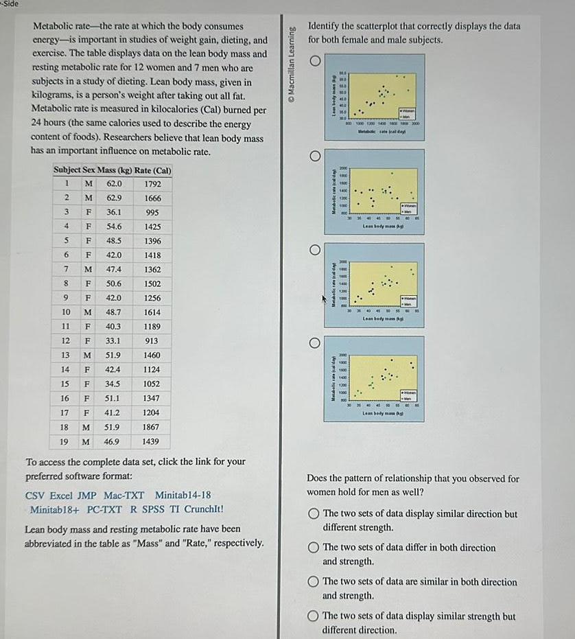
Side Metabolic rate the rate at which the body consumes energy is important in studies of weight gain dieting and exercise The table displays data on the lean body mass and resting metabolic rate for 12 women and 7 men who are subjects in a study of dieting Lean body mass given in kilograms is a person s weight after taking out all fat Metabolic rate is measured in kilocalories Cal burned per 24 hours the same calories used to describe the energy content of foods Researchers believe that lean body mass has an important influence on metabolic rate Subject Sex Mass kg Rate Cal 1 M 62 0 2 62 9 3 36 1 4 54 6 5 48 5 42 0 M 47 4 F 50 6 9 F 42 0 10 M 48 7 11 F 40 3 12 F 33 1 13 M 51 9 14 F 42 4 15 F 34 5 16 F 51 1 17 F 41 2 18 M 51 9 19 M 46 9 in 6 7 8 MF FFF 1792 1666 995 1425 1396 1418 1362 1502 1256 1614 1189 913 1460 1124 1052 1347 1204 1867 1439 To access the complete data set click the link for your preferred software format CSV Excel JMP Mac TXT Minitab14 18 Minitab18 PC TXT R SPSS TI CrunchIt Lean body mass and resting metabolic rate have been abbreviated in the table as Mass and Rate respectively Macmillan Learning Identify the scatterplot that correctly displays the data for both female and male subjects O O Leanbody Metaboliccate da Metabolic rate ada 563 80 100 100 100 100 2000 Metabolic tale calday 1000 1800 1400 1200 smo 1400 1 200 1000 30 31 2000 1300 1900 1400 1300 1000 10 LHH BHN mang 44 Lean body mas re no 105 Lean body mas g Does the pattern of relationship that you observed for women hold for men as well The two sets of data display similar direction but different strength The two sets of data differ in both direction and strength The two sets of data are similar in both direction and strength The two sets of data display similar strength but different direction

1 ep ncy 5 2 5 0 S 9 0 2 7 2 ep mcy 7 2 Asymmetry index 0 107 0 013 0 074 0 002 0 012 0 055 0 019 0 050 0 045 0 009 0 001 Asymmetry index 0 047 0 021 0 001 0 004 0 006 0 015 0 020 0 027 To access the complete data set click the link for your preferred software format Excel Minitab14 18 Minitab18 JMP SPSS TI R Mac TXT PC TXT CSV CrunchIt Macmillan Learning Taking a long time to fall asleep could indicate a greater level of sleep disturbance so sleep latency should be the explanatory variable Display the data for both nights in the same scatterplot using different symbols for each night Alternatively you can plot the data in two side by side scatterplots that use the same x and y scales to make both patterns truly comparable Identify the scatterplot that displays the data for both nights on the same scatterplot using different symbols for each night O 410 And

Most people think that the normal adult body temperature is 98 6 F In a more recent study researchers reported that a more accurate figure may be 98 1 F Furthermore the standard deviation appeared to be around 0 8 F Assume that a Normal model is appropriate Complete parts a through c below a In what interval would you expect most people s body temperatures to be Explain Select the correct choice below and fill in the answer box es to complete your choice A Using the 68 95 99 7 Rule about 95 of the body temperatures are expected to be between 96 5 F and 99 7 F Use ascending order Round to one decimal place as needed OB Using the 68 95 99 7 Rule about 95 of the body temperatures are expected to be less than Round to one decimal place as needed OC Using the 68 95 99 7 Rule about 95 of the body temperatures are expected to be at least Round to one decimal place as needed b What fraction of people would be expected to have body temperatures above 98 6 F Round to two decimal places as needed F F

de Algal blooms can have negative effects on an ecosystem by dominating its phytoplankton communities Gonyostomum semen is a nuisance alga infesting many parts of northern Europe Could the overall biomass of G semen be controlled by grazing zooplankton species A research team examined the relationship between the net growth rate of G semen and the number of Daphnia magna grazers introduced in test tubes A net growth rate was computed by comparing the initial and final abundances of G semen in the experiment with a negative value indicating a decrease in abundance Here are the findings ZEL N be of gr az S N et 0 wt h ra te 1 2 3 4 5 6 1 9 2 5 2 2 3 9 4 1 4 3 To access the complete data set click the link for your preferred software format Excel Minitab14 18 Minitab18 JMP SPSS TI R Mac TXT PC TXT CSV CrunchIt 1 From graphs in K Lebret et al Grazing resisitance allows bloom ormation and may explain invasion success of Gonyostomum semen Limnology and Oceanography 57 2012 pp 727 734 Hoi 10 4319 lo 2012 57 3 0727 Macmillan Learning Make a scatterplot of number of grazers and net growth rate Do you think that D magna is an effective grazer of the G semen alga The nonlinear relationship indicates that D magna is not an effective grazer of the G semen alga The positive linear relationship indicates that D magna is not an effective grazer of the G semen alga The negative linear relationship indicates that D magna is an effective grazer of the G semen alga The negative linear relationship indicates that D magna is not an effective grazer of the G semen alga The positive linear relationship indicates that D magna is an effective grazer of the G semen alga

Macmillan Learning The scatterplot shows the age in months at which a child begins to Gesell Adaptive Score for each of 21 children 2 sets of 2 children happen to have the same values Gesell Adaptive Score 120 110 100 90 80 70 60 50 L 5 10 15 20 25 30 35 40 45 Age at first word months One child clearly falls outside of the overall pattern of the scatterplot and therefore might be an outlier The possible outlier is the child with O age 26 months and score 71 age 17 months and score 121 age 7 months and score 113 O age 42 months and score 57 1 These data were originally collected by L M Linde of UCLA but were first published by M R Mickey O J Dunn and V Clark Note on the use of stepwise regression in detecting outliers Computers and biomedical Research 1 1967 pp 105 111 The data have been used by several authors These are taken from N R Draper and J A John Influential observations and outliers in regression Technometires 23 1981 pp 21 26

Side by Side College freshmen involved in a dating relationship agreed to participate in a nine month long study Every two weeks participants answered a detailed questionnaire about their relationship and their emotional well being Over the course of the study 26 of the participants experienced a breakup The average distress of these 26 participants at the time of breakup 0 weeks and over the following 10 weeks was assessed from their questionnaire answers The table shows the findings in a scientific publication Time since brea kup wee ks Aver age distr ess unit less score 0 2 6 10 3 3 3 1 2 9 2 6 CSV Excel JMP Mac TXT Minitab14 18 Minitab18 PC TXT R SPSS TI CrunchIt P Eastwick et al Mispredicting distress following romantic breakup Revealing the time course of the affective forecasting error Journal of Experimental Social Psychology 44 2008 pp 800 807 doi 10 1016 j jesp 2007 07 001 Macmillan Learning How strong is the correlation between average distress and time since breakup Explain how the value for r matches your description from the scatterplot The correlation is close to 1 so it is very weak and does not represent the same direction as the scatterplot The correlation is close to 1 so it is very strong and represents the same direction as the scatterplot The correlation is close to 0 so it is very weak and represents the same direction as the scatterplot The correlation is close to 1 so it is very strong and does not represent the same direction as the scatterplot If we had measured time since breakup in days rather than weeks how would that difference affect r The correlation would changed from weeks to days if the units

olic rate the rate at which the body consumes is important in studies of weight gain dieting and se The table displays data on the lean body mass and metabolic rate for 12 women and 7 men who are Is in a study of dieting Lean body mass given in ams is a person s weight after taking out all fat lic rate is measured in kilocalories Cal burned per rs the same calories used to describe the energy I of foods Researchers believe that lean body mass important influence on metabolic rate ubject Sex Mass kg Rate Cal 1 M 62 0 1792 M 62 9 1666 F 36 1 995 F 54 6 1425 F 48 5 1396 6 F 42 0 1418 7 M 47 4 1362 8 F 50 6 1502 9 F 42 0 1256 10 M 48 7 1614 11 F 40 3 1189 12 F 33 1 913 13 M 51 9 1460 14 F 42 4 1124 F 34 5 1052 16 F 51 1 1347 17 F 41 2 1204 18 M 51 9 1867 9 M 46 9 1439 2 3 4 5 15 s the complete data set click the link for your software format cel JMP Mac TXT Minitab14 18 18 PC TXT R SPSS TI CrunchIt y mass and resting metabolic rate have been ed in the table as Mass and Rate respectively Macmillan Learning Make a scatterplot of the data for the female subjects Which is the explanatory variable rate O subject number mass sex Explain why the subject number is not part of the scatterplot O Subject number is an index variable and thus contains no data A scatterplot cannot graph more than one categorical variable A scatterplot cannot display numbers without units O The subject number is not appropriate to graph the subjects were anonymous

ne activity is known to be affected by temperature A examnied the activity rate in micromoles per second s of the digestive enzyme acid phosphatase in vitrol ving temperatures measured in kelvins K The gs are displayed in the following table For nce the range of 253 to 298 K corresponds to y 25 to 80 degrees Celsius or 77 to 176 es Fahrenheit emperat ure K 298 298 298 303 303 303 308 308 308 313 313 313 Rate u mol s 348 353 353 353 0 04 0 05 0 05 0 08 0 08 0 08 0 11 0 13 0 11 0 18 0 20 0 19 emperat ure K 338 1 05 338 1 10 338 1 06 343 0 96 343 0 98 343 0 99 348 0 72 348 0 73 0 75 0 54 0 58 0 62 Rate u mol s Temperat ure K 318 318 318 323 323 323 323 328 328 333 333 333 Rate mol s To access the complete data 0 34 0 34 0 35 0 47 software 0 48 format 0 48 Excel 0 48 0 78 0 79 0 97 0 98 1 03 set click the link for your preferred Minitab14 18 Minitab 18 JMP SPSS TI R Mac TXT PC TXT CSV CrunchIt Macmillan Learning Describe the form of the relationship It is not linear Explain why the form of the relationship makes sense The relationship curves upward and then levels off This makes sense as temperatures can increase the speed of chemical reactions to a point and then the impact plateaus at a certain point O The relationship is curved This makes sense because temperature impacts on the speed of chemical reactions is cyclical in nature as temperature increases The relationship is curvilinear This makes sense because increasing temperatures increase the speed of chemical reactions at graduating temperature levels The relationship is curved This makes sense as temperatures can increase the speed of chemical reactions to a point but very high temperatures can have negative effects

yme activity is known to be affected by temperature A y examnied the activity rate in micromoles per second l s of the digestive enzyme acid phosphatase in vitrol rying temperatures measured in kelvins K The ings are displayed in the following table For rence the range of 253 to 298 K corresponds to ghly 25 to 80 degrees Celsius or 77 to 176 rees Fahrenheit Temperat ure K 298 298 298 303 303 303 308 308 308 313 313 313 Temperat ure K 338 338 338 343 343 343 348 348 348 353 353 353 Rate u mol s 0 04 0 05 0 05 0 08 0 08 0 08 0 11 0 13 0 11 0 18 0 20 0 19 Rate u mol s 1 05 1 10 1 06 0 96 0 98 0 99 0 72 0 73 0 75 0 54 0 58 0 62 Temperat ure K 318 318 318 323 323 323 323 328 328 333 333 333 Rate mol s To access the complete data set click the link for your 0 34 0 34 0 35 preferred 0 47 software 0 48 format 0 48 Excel 0 48 0 78 0 79 0 97 0 98 1 03 Minitab14 18 Minitab18 JMP SPSS TI R Mac TXT PC TXT CSV CrunchIt a activity on temperature Macmillan Learning Make a scatterplot Which is the explanatory variable The explanatory variable is temperature The explanatory variable is enzyme activity rate The explanatory variable is enzyme activity rate The explanatory variable is temperature

You have data for many individuals on their walking speed and their heart rate after a 10 minute walk You expect to see no association O a negative association O a positive association O very little association

Cassandra has been researching preparation courses for the Graduate Writing Test They are expensive courses and she wants to select the course associated with the best outcome that is higher test scores The first course she researched Course A reported a mean score of M 72 with a standard deviation of s 15 for their graduates The web page for the second course Course B only provided a sample of scores for their most recent graduates n but no statistics The scores for course B were 100 77 87 84 92 Formula for the mean Image result for mean formula Question 24 Compute the mean for Course B

A recent poll was taken from SJSU college students asking their political affiliation either Republican R Democrat Independent I The following responses are from a sample of 40 SJSU students R 1 D D D D R K R DI R Political Affiliation IDD DR D D R R D D R RD D R Proportion D D D R R D Complete the frequency distribution table for these data Be sure your frequencies sum to 40 R Political Affiliation first column f second column proportion third column round to the 1 decimal place D

Use the Normal model N 98 17 for the IQs of sample participants a What IQ represents the 18th percentile b What IQ represents the 90th percentile c What s the IQR of the IQs a The IQ representing the 18th percentile is Round to one decimal place as needed

R D D D D 2 D O 20 O 30 O 70 R O 50 D O 80 Question 15 R R Question 16 20 D D D D R D R R D D R D D R D D D What percentage of respondents identify their political affiliation as Republican R K D R D What percentage of respondents identify their political affiliation as either Democrat or Republican Cannot be determined with the given information

NFL data from the 2019 football season reported the number of yards gained by each of the league s 508 receivers The mean is 253 761 yards with a standard deviation of 312 358 yards Complete parts a through c below Click the icon to view a histogram of the receivers yards a According to the Normal model what percent of receivers would you expect to gain more yards than 2 standard deviations above the mean number of yards Type an integer or a decimal rounded to one decimal place as needed

Some IQ tests are standardized to a Normal model N 100 11 a What cutoff value bounds the highest 5 of all IQs b What cutoff value bounds the lowest 35 of the IQs c What cutoff values bound the middle 80 of the IQs a The cutoff value is Round to one decimal place as needed

Companies who design furniture for elementary school classrooms produce a variety of sizes for kids of different ages Suppose the heights of kindergarten children can be described by a Normal model with a mean of 39 2 inches and standard deviation of 1 9inches a What fraction of kindergarten kids should the company expect to be less than 35 inches tall About of kindergarten kids are expected to be less than 35 inches tall Round to one decimal place as needed

a Draw and label the Normal model OA levels of women can be described by a Normal model with a mean of 188 mg dL and a standard deviation of 28 Complete parts a through e 10 174 211 230 60 Round to two decimal places as needed SON 997 104 32 160 188 215 241 272 b What percent of women do you expect to have cholesterol levels over 210 mg dL 00 20 95 26 22 100

Use the Normal model N 100 16 describing IQ scores to answer the following a What percent of people s IQs are expected to be over 80 b What percent of people s IQs are expected to be under 90 c What percent of people s IQs are expected to be between 116 and 128 a Approximately of people s IQs are expected to be above 80 Round to one decimal place as needed

The just is standar 200 10 a mai model with a mean of 100 and a standard deviation of 20 a Choose the model for these IQ scores that correctly shows what the 68 95 99 7 rule predicts about the scores OB 63 PIO 95 997 30 4050 00 100 120 140 100 20 99 pre b In what interval would you expect the central 99 7 of the IQ scores to be found and Using the 68 95 99 7 rule the central 99 7 of the IQ scores are between Type integers or decimals Do not round Q Q 95 03 1 30 40 60 BO 100 120 140 160 20 G O c 63 PIC 95 99 50 00 100 120 140 100 Q S

The first Stat exam had a mean of 85 and a standard deviation of 4 points the second had a mean of 70 and a standard deviation of 15 points Reginald scored an 85 on the first test and a 90 on the second Sara scored a 93 on the first test but only a 65 on the second Although Reginald s total score is higher Sara feels she should get the higher grade Explain her point of view Select the correct choice below and fill in the answer boxes to complete your choice Round to two decimal places as needed OA The standardized score of Sara s best test is while the standardized score of Reginald s best test is OB The sum of Sara s standardized scores is while the sum of Reginald s standardized scores is When the test scores are standardized Sara did better than Reginald When the test scores are standardized Sara did better than Reginald

An incoming MBA student took placement exams in economics and mathematics In economics she scored 82 and in math 90 The overall results on the economics exam had a mean of 71 and a standard deviation of 7 while the mean math score was 68 with a standard deviation of 11 On which exam did she do better compared with the other students Since she scored standard deviations Round to two decimal places as needed CLES the mean in economics and standard deviations the mean in mathematics she did better on the exam

One season baseball player A hit 65 home runs During a different season baseball player B hit 71 home runs How does the performance of player A compare to the performance of player B The table available below shows the means and standard deviations for the number of home runs scored by all players with at least 502 plate appearances in their respective seasons Use these to determine whose home run feat was more impressive Click the icon to view the means and standard deviations for the two seasons The Z score for player A ZA is Round to two decimal places as needed than the z score for player B Z so the feat by player was more impressive

A town s January high temperatures average 38 F with a standard deviation of 10 while in July the mean high temperature is 77 and the standard deviation is 0 In which month is it more unusual to have a day with a high temperature of 57 Explain Select the correct choice below and fill in the answer boxes within your choice Round to three decimal places as needed OA It is more unusual to have a day with a high temperature of 57 in January A high temperature of 57 in January is standard deviations above the mean and a high temperature of 57 in July is only standard deviations below the mean OB It is more unusual to have a day with a high temperature of 57 in July A high temperature of 57 in July is standard deviations below the mean and a high temperature of 57 in January is only standard deviations above the mean

People with 2 scores of 2 5 or above on a certain aptitude test are sometimes classified as geniuses If aptitude test scores have a mean of 100 and a standard deviation of 12 points what is the minim aptitude test score needed to be considered a genius The minimum aptitude test score needed to be considered a genius is points Type an integer or a decimal Do not round CIT